Titanic - Random Forest
In the last publication from StatCityPro a decision tree classification model was created with the aim of predicting if a passenger on the Titanic survived or died. Cross validation was used with an accuracy of 80.79% achieved.
In this new publication a Random Forest model is used to try and improve the accuracy. The data used is the same as the data which was being used at the end of the previous publication. (total, train_val, train_test_val). Therefore, feature engineering has already been carried out with the data ready for model creation.
2) Packages
The following packages are used in this publication.
library(dplyr)
library(tidyr)
library(ggplot2)
library(knitr)
library(DT)
library(purrr)
library(corrplot)
library(randomForest)
library(caret)
library(rpart)
library(rpart.plot)
3) Loading the Data
setwd("~/Documents/Machine Learning/15. Hugo/academic-kickstart-master/content/en/post/Titanic-RF")

total <- read.csv("total2.csv")

total <- total[,-1]

train_val <- read.csv("train_val.csv")

train_test_val <- read.csv("train_test_val.csv")
The variables of Title and Age Group are changed to factors.
train_val$Title <- as.factor(train_val$Title)
train_val$Age.Group <- as.factor(train_val$Age.Group)
train_val$Survived <- as.factor(train_val$Survived)
4) Variables and Data
The data base total has 1,309 observations and 16 variables. Of these 1,309 observations, 891 are training data and 418 are testing data.
To train the model the 891 training observations are used, and are divided into two groups. The first group is train_val which has 714 observations. This group is used to train the model. Then the model is tested using the second group train_test_val which acts as a preliminary testing group. After the feature engineering that took place in the part 1 publication these data bases only have seven variables.
| Variable | Description |
|---|---|
| Survived | Survived (1) or Died (0) |
| Pclass | Social class of passenger |
| Title | Title of passenger |
| Sexo | Sex of passenger |
| Age Group | Age group of passenger |
| Family_size | Number of family members on Titanic |
| Embarked | Port of embarkation |
5) What is a Random Forest Model?
A Random Forest is a collection of decision trees that are joined together in a forest. This collection of trees is what makes a Random Forest Model more reliable than a Decision Tree Model. Each tree gives a classification of survived or deceased for each observation. For each observation the final result is the most frequent classification. For example in a model with 500 trees, if 300 predict that an observation survived and 200 predict that they died, the observation is classified as survived.
6) Creating the Model
The model is created using survived as the dependent variable and the other six variables as independent variables. The model is ran against the train_val data and obtains an accuracy of 83.47% (100 - 16.53 (error rate)). The model uses 500 trees with two variables tested at each node. Further on these settings are verified to check the model can not be improved with different settings.
set.seed(1234)
rf_model <- randomForest(Survived ~ Pclass + Title + Sex + Embarked + Family_size + Age.Group, data = train_val, ntree = 500)


rf_model
##
## Call:
## randomForest(formula = Survived ~ Pclass + Title + Sex + Embarked + Family_size + Age.Group, data = train_val, ntree = 500)
## Type of random forest: classification
## Number of trees: 500
## No. of variables tried at each split: 2
##
## OOB estimate of error rate: 16.53%
## Confusion matrix:
## 0 1 class.error
## 0 409 31 0.07045455
## 1 87 187 0.317518256.1) Number of Trees
In this section the number of trees in the model is reviewed to see if it needs to be increased. A table is created to show the error rate for each of the 500 trees. For each tree there are tree error rates:
- for values of 0 (somebody who died)
- for values of 1 (somebody who survived)
- for all values (people who died and survived)
These error rates are graphed. It is hoped that before the 500th tree the error rate will have stabilised with a flat line present on the graph.
oob.error.data <- data.frame(
  Trees=rep(1:nrow(rf_model$err.rate), times=3),
  Type=rep(c("OOB", "0", "1"), each=nrow(rf_model$err.rate)),
  Error=c(rf_model$err.rate[,"OOB"],
          rf_model$err.rate[,"0"],
          rf_model$err.rate[,"1"]))
ggplot(data=oob.error.data, aes(x=Trees, y=Error)) +
geom_line(aes(color=Type))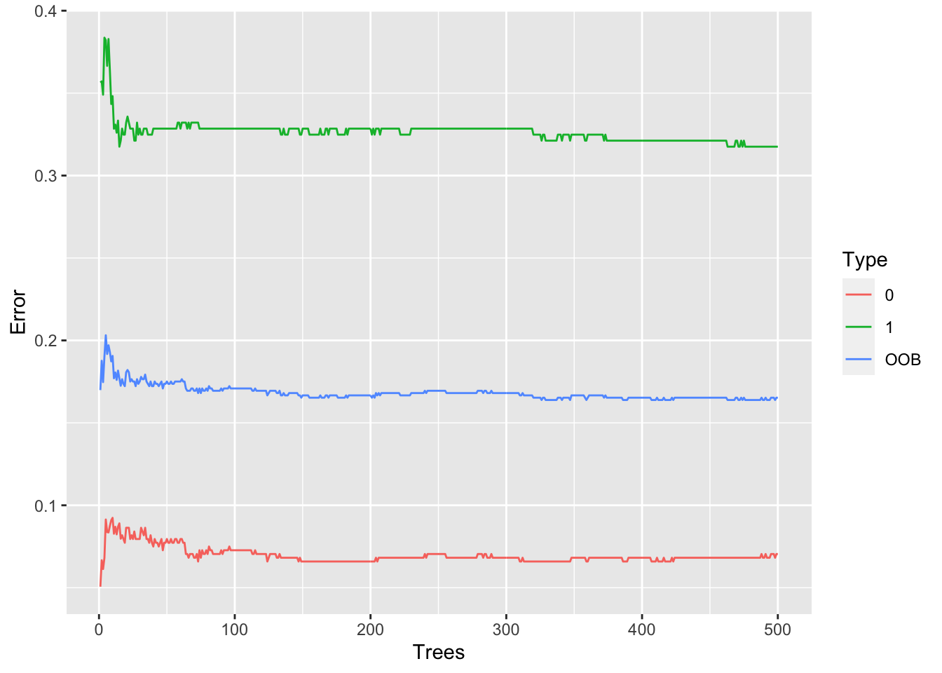
In the above graph it is clear that the error rate stabilises before the 500th tree. This means that it is not necessary to add more trees to the model, as they would not reduce the error rate any more.
6.2) Number of Variables
In this section a test is run to see how many variables should be tested at each node in the model. Currently, two variables are tested.
In oob.values it is shown that mtry=2, with two tested variables, gives the lowest error value (0.1666667) and therefore is the value that is used in the model.
oob.values <- vector(length = 10)
for(i in 1:10) {
  temp.model <- randomForest(Survived ~ Pclass + Title + Sex + Embarked + Family_size + Age.Group, data = train_val, mtry=i, ntree=500)
  oob.values[i] <- temp.model$err.rate[nrow(temp.model$err.rate),1]
  }

oob.values
## [1] 0.1918768 0.1666667 0.1778711 0.1806723 0.1764706 0.1778711 0.1806723
## [8] 0.1806723 0.1792717 0.17366956.3) Variable Importance
The Gini value can be used to determine which variable are the most and least important in the model. The below table and graph show that the variables Age_Group and Embarked have a low importance in the model. Therefore a new model is tried without these two variables.
importance(rf_model)## MeanDecreaseGini
## Pclass 33.40132
## Title 62.14757
## Sex 42.51139
## Embarked 11.08408
## Family_size 22.26955
## Age.Group 11.74166varImpPlot(rf_model)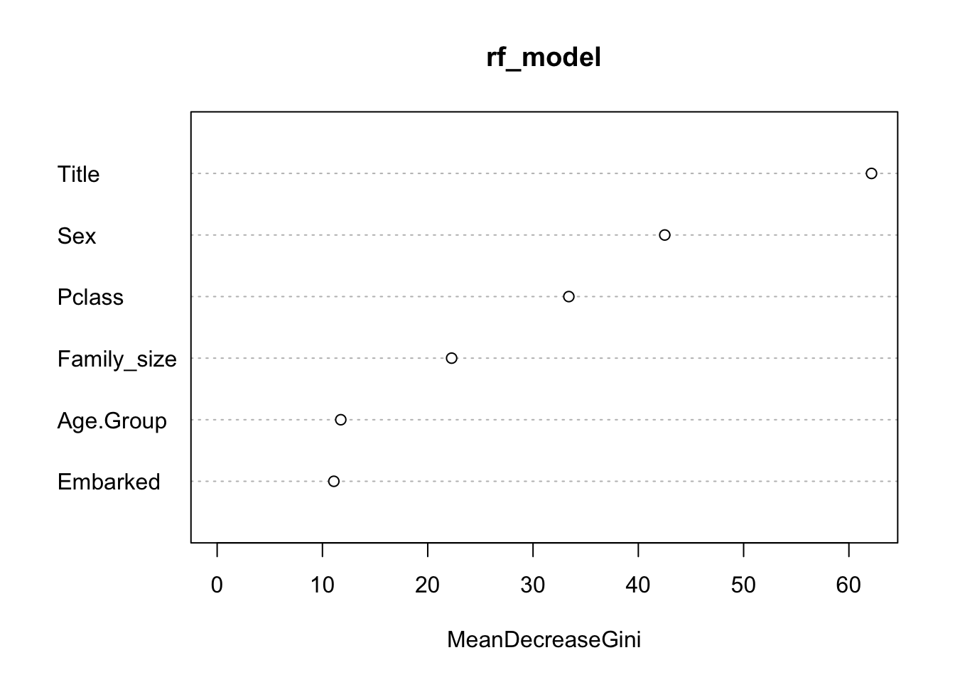
7) New Model
A new model is created without the variables for Age.Group and Embarked. The settings of 500 trees and two variables at each node are used.
However, when the model is run using the train_val data it seems that the two removed variables are in fact needed in the model as without them the accuracy is reduced to 82.63% (100 - 17.37% (error rate)). Therefore, the first model with all of the independent variables is used as the final model.
train_val1=train_val[,c(-4,-6)]

train_test_val1=train_test_val[,c(-4,-6)]
set.seed(1234)
rf_model2 <- randomForest(Survived ~ Pclass + Title + Sex + Family_size, data = train_val1, ntree=500)
rf_model2##
## Call:
## randomForest(formula = Survived ~ Pclass + Title + Sex + Family_size, data = train_val1, ntree = 500)
## Type of random forest: classification
## Number of trees: 500
## No. of variables tried at each split: 2
##
## OOB estimate of error rate: 17.37%
## Confusion matrix:
## 0 1 class.error
## 0 387 53 0.1204545
## 1 71 203 0.2591241varImpPlot(rf_model2)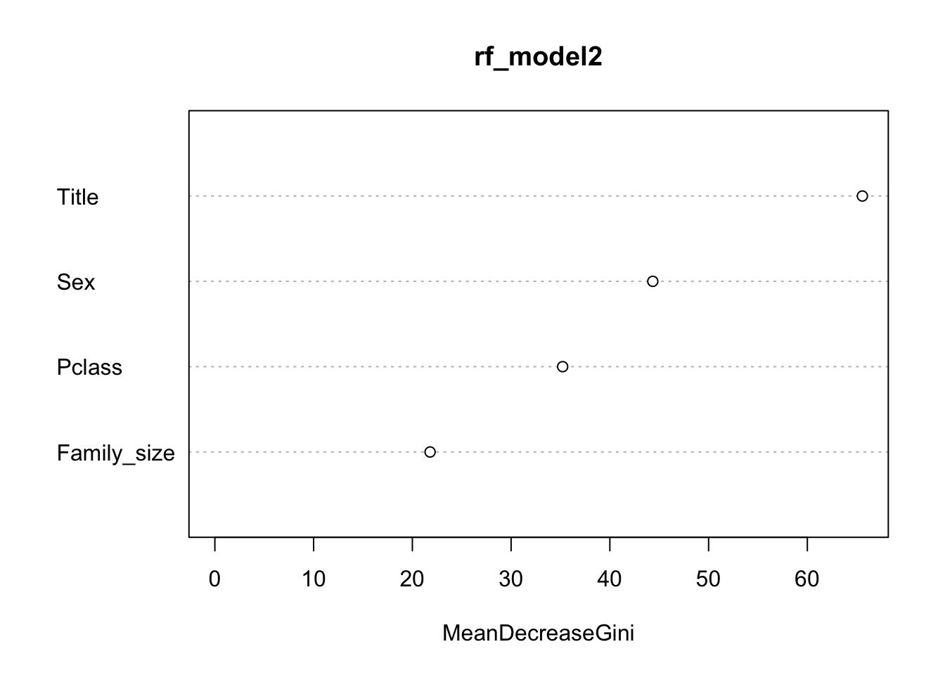
8) Testing the Model
In this section the model is tested using the train_test_val data. In order to prepare this data some variables are converted to factors. The model is then run with the dependent variable hidden to predict which people survived or died. The predictions are then compared to the real data in a confusion matrix with the model achieving an accuracy of 83.05% and a kappa value of 0.6316.
train_test_val$Title <- as.factor(train_test_val$Title)
train_test_val$Age.Group <- as.factor(train_test_val$Age.Group)
train_test_val$Survived <- as.factor(train_test_val$Survived)
set.seed(1234)
rf_predictions <- predict(rf_model, train_test_val)
confusionMatrix(train_test_val$Survived, rf_predictions)## Confusion Matrix and Statistics
##
## Reference
## Prediction 0 1
## 0 99 10
## 1 20 48
##
## Accuracy : 0.8305
## 95% CI : (0.767, 0.8826)
## No Information Rate : 0.6723
## P-Value [Acc > NIR] : 1.683e-06
##
## Kappa : 0.6316
##
## Mcnemar's Test P-Value : 0.1003
##
## Sensitivity : 0.8319
## Specificity : 0.8276
## Pos Pred Value : 0.9083
## Neg Pred Value : 0.7059
## Prevalence : 0.6723
## Detection Rate : 0.5593
## Detection Prevalence : 0.6158
## Balanced Accuracy : 0.8298
##
## 'Positive' Class : 0
## 9) Conclusion
In this publication a Random Forest Model has been created to predict if somebody survived or died on board the titanic. It was hopped that the model would improve on the accuracy achieved using a decision tree model in a previous publication. The accuracy was improved with the Random Forest Model achieving an accuracy of 83.05% in comparison to the 80.79% of the Decision Tree Model. 500 trees were used with two variables tested at each node. Thank you for taking the time to read this publication and hopefully it has been of use.