Titanic - Who Survived? - Part 2
This publication will follow on from Part one on the Titanic to conduct data analysis for the passengers onboard and to create a classification decision tree model to predict if a passenger survived or died. Part one covered the data preparation process.
2) Packages
The following packages are used in this publication.
library(dplyr)
library(readr)
library(tidyr)
library(ggplot2)
library(knitr)
library(DT)
library(purrr)
library(corrplot)
library(randomForest)
library(caret)
library(rpart)
library(rpart.plot)
3) Data Exploration
With the data already prepared in part 1 the next step is to carry out some data exploration to better understand the data’s characteristics. Only the train data is be used in this data exploration section.
setwd("~/Documents/Machine Learning/15. Hugo/academic-kickstart-master/content/en/post/Titanc-part2")


total <- read_csv("total2.csv")

total <- total[,-1]

test <- read.csv("test.csv")

train <- read.csv("train.csv")
3.1) Pclass
The below graph shows the survival of passengers in each of the three classes. Red represents passengers that died, and blue passengers that survived. The white line is the average survival rate for passengers in the training data (38.38%).
First class passengers had a survival rate higher than the average. Second class passengers followed this trend, all be it to a lesser degree with a survival rate of close to 50%. In comparison third class passengers had a lower survival rate of 25%.
ggplot() +

  geom_bar(data = total %>% filter(group == 'train'), aes(Pclass, fill = as.factor(Survived)), position = 'fill') +

  geom_hline(yintercept = 0.3838, col = "white", lty=2, size=2) +

    scale_fill_brewer(palette="Set1") +

  ylab("Survival Rate") +

  xlab("Class") +

  ggtitle("Survival Rate by Class") +

  labs(fill = "Survived") +

  theme_minimal()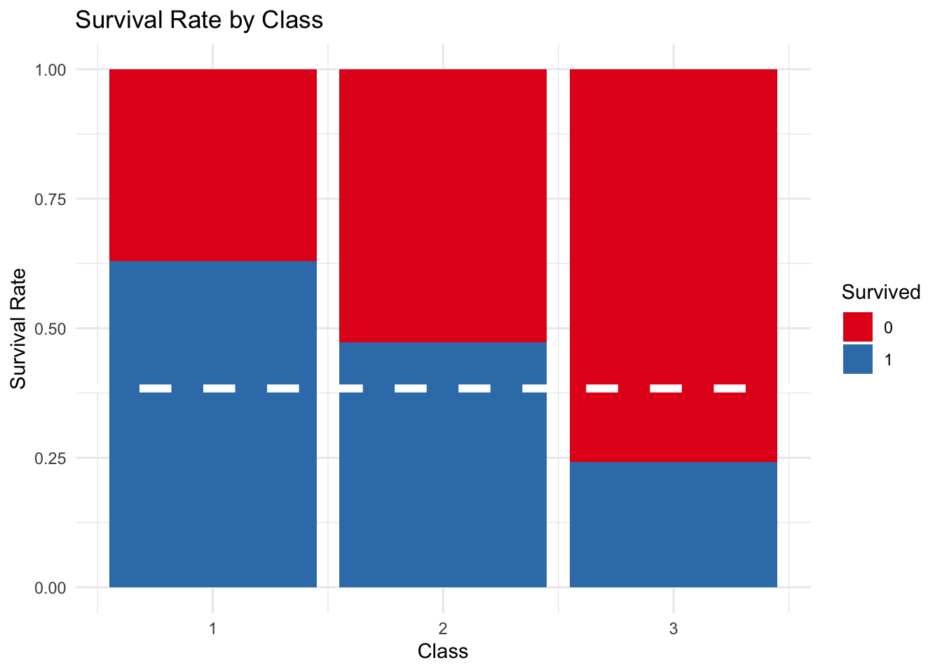
5.2) Title
The following graph highlights how passengers with the tile ‘Mr’ had a very low survival rate. In comparision a child with the title ‘Master’ or an adult woman with the title “Miss” had a greater chance of survival with survival rates of close to 70%.
ggplot() +

  geom_bar(data = total %>% filter(group == 'train'), aes(Title, fill = as.factor(Survived)), position = 'fill') +

  geom_hline(yintercept = 0.3838, col = "white", lty=2, size=2) +

    scale_fill_brewer(palette="Set1") +

  ylab("Survival Rate") +

  ggtitle("Survival Rate by Title") +

  labs(fill = "Survived") +

  theme_minimal()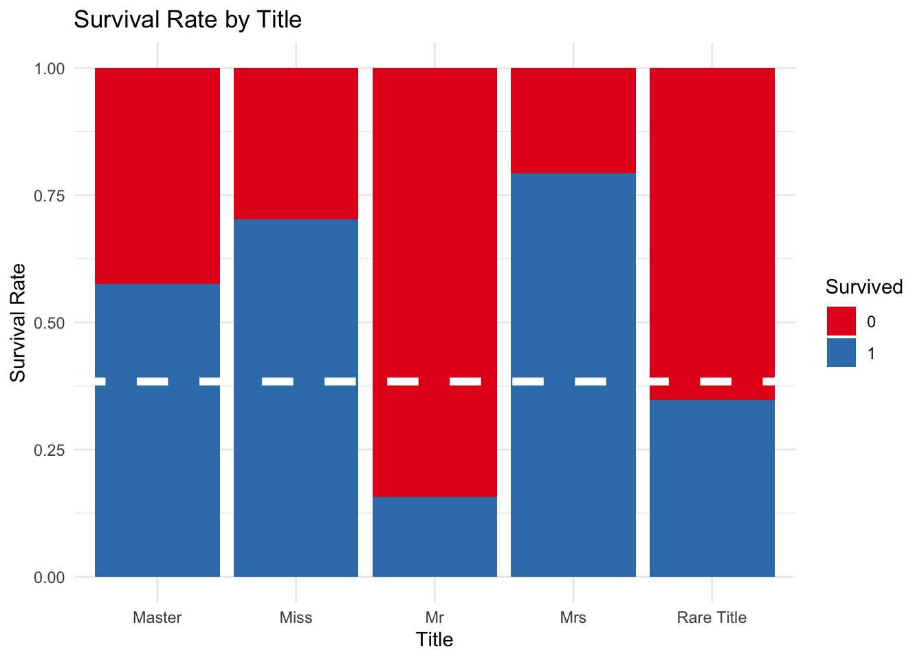
5.3) Port
There were three ports of embarkation: Southampton, Great Britain; Cherborg, France; and Queenstown, Ireland. There is not that much variation in the survival rates of passengers from different ports, however, passengers from Cherborg had the highest survival rate.
ggplot(total %>% filter(group=="train"), aes(Embarked, fill=as.factor(Survived))) +

  geom_bar(position = "fill") +

  scale_fill_brewer(palette="Set1") +

  ylab("Survival Rate") +

  geom_hline(yintercept=0.38, col="white", lty=2, size=2) +

  ggtitle("Survival Rate by Emarking Point") +

  labs(fill = "Survived") +

  theme_minimal()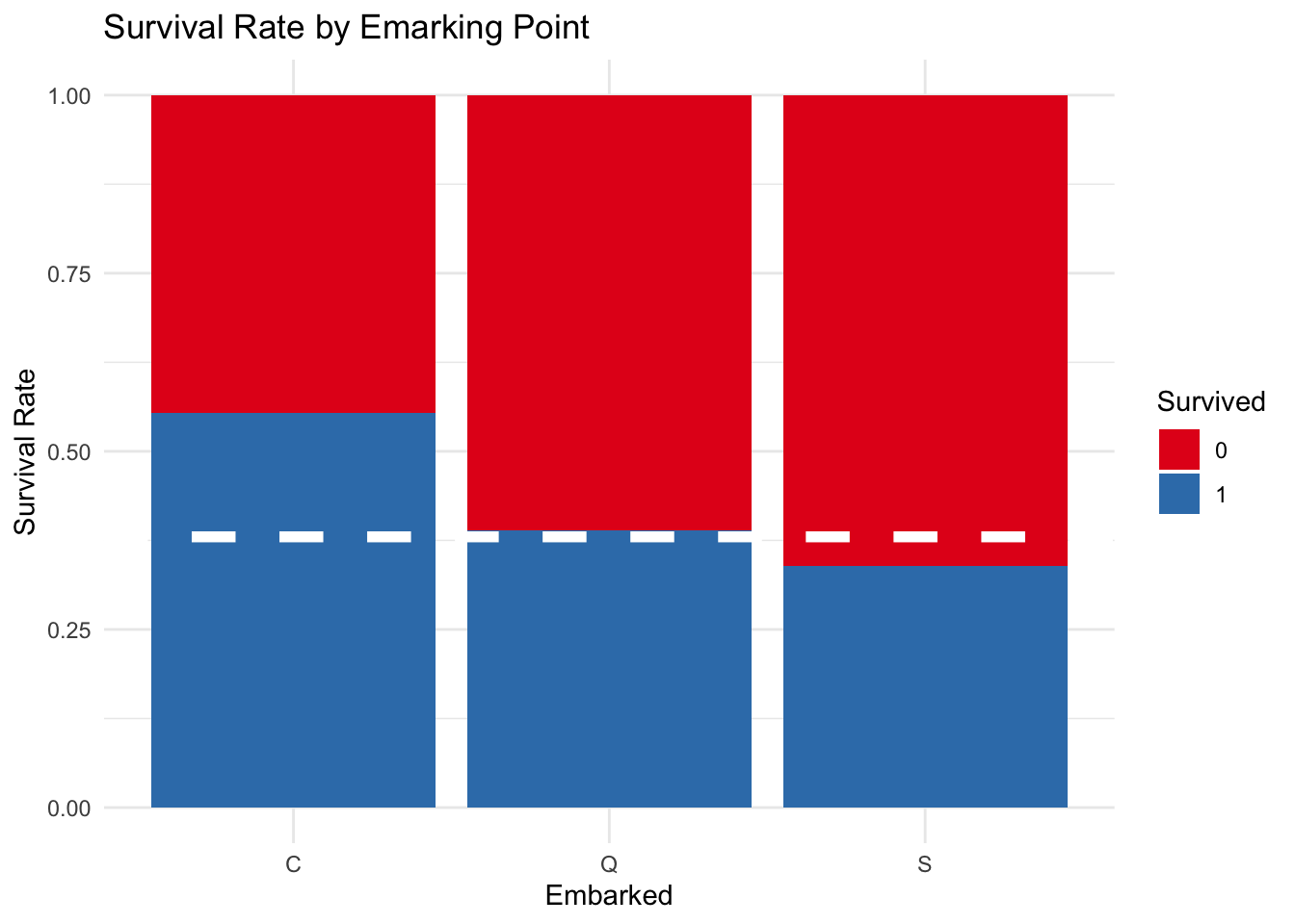
5.4) Fare and Class
The below graph show the relationship between survival and fare. The graph suggests that passengers with a more expensive ticket were more likely to survive. For example, there is a higher concentration of tickets with a cost of more than £50, found in those passengers who survived.
ggplot(total %>% filter(group=="train"), aes(Fare, Survived)) +

  geom_point() +

  ylab("Survival Rate") +

  ggtitle("Survival vs. Fare") +

  theme_minimal()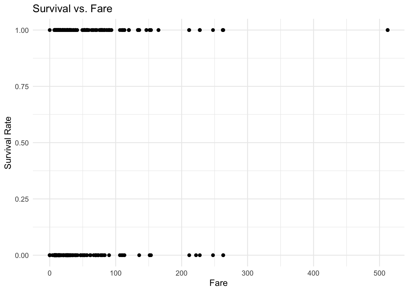
Class can also be plotted by fare with this graph suggesting that there is potentially a strong correlation between class and fare.
ggplot(total %>% filter(group=="train"), aes(Pclass, Fare)) +

  geom_point() +

  ylab("Fare (£)") +

  xlab("Class") +

  ggtitle("Class vs. Fare") +

  theme_minimal()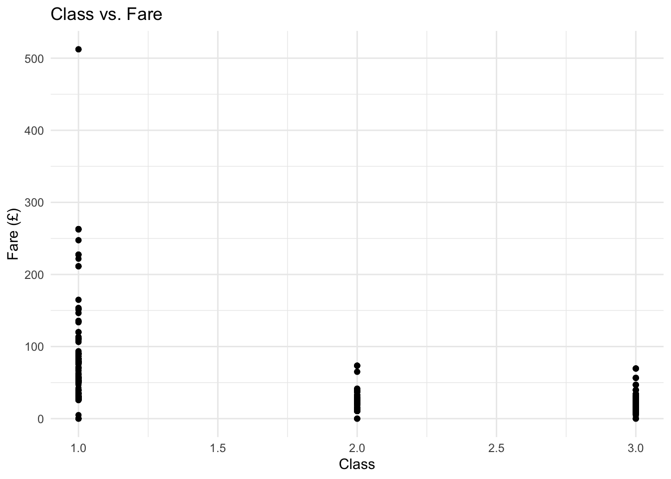
5.4.1) Over Correlation
Following on from the above suggestion of a correlation between class and fare the correlation for these two variables is calculated. The below graphic shows there is a negative correlation of 0.55 between these two variables. This correlation could be detrimental to the model with class and fare both having the same impact on the dependent variable and multicollinearity occurring. Therefore fare will not be included in the model.
tbl_corr <- total %>%

  filter(group=="train") %>%

  select(-PassengerId, -SibSp, -Parch) %>%

  select_if(is.numeric) %>%

  cor(use="complete.obs") %>%

  corrplot.mixed(tl.cex=0.85)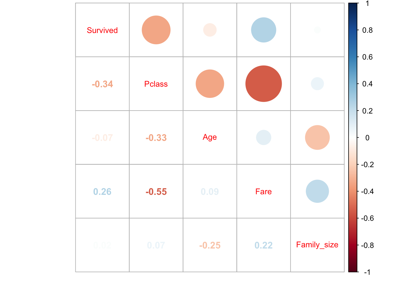
5.5) Sex
This graph shows that females had a higher rate of survival that males. Almost 75% of the females survived in comparison with close to 23% of the males.
ggplot(total %>% filter(group=="train"), aes(Sex, fill=as.factor(Survived))) +

  geom_bar(position = "fill") +

  scale_fill_brewer(palette="Set1") +

  ylab("Survival Rate") +

  geom_hline(yintercept=0.38, col="white", lty=2, size=2) +

  ggtitle("Survival Rate by Sex") +

  labs(fill = "Survived") +

  theme_minimal()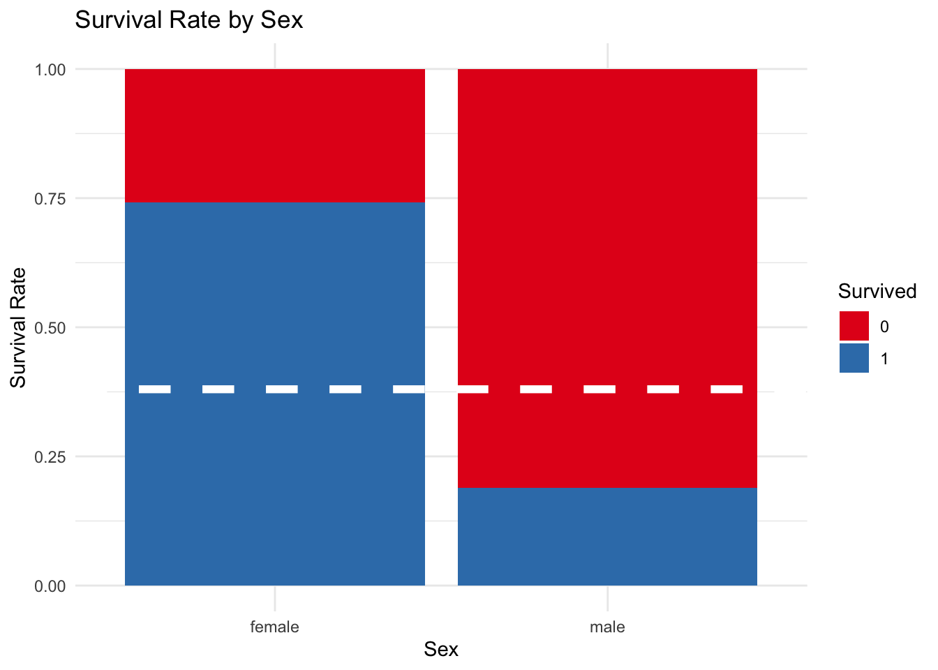
5.5.1) Sex y Class
The following graph shows how sex had a very strong impact on the chances of survival. To be a female from first or second class almost was a characteristic of survival, and almost 50% of the females in third class survived. In comparison to these figures the survival rate for males, without taking into account their class, was never higher than the average survival rate for all passengers.
ggplot(total %>% filter(group=="train"), aes(Pclass, fill=as.factor(Survived))) +

  facet_wrap(~Sex, scale = "free") +

  geom_bar(position = "fill") +

  scale_fill_brewer(palette="Set1") +

  ylab("Survival Rate") +

  geom_hline(yintercept=0.38, col="white", lty=2, size=2) +

  ggtitle("Survival Rate by Sex and Class") +

  labs(fill = "Survived") +

  theme_minimal()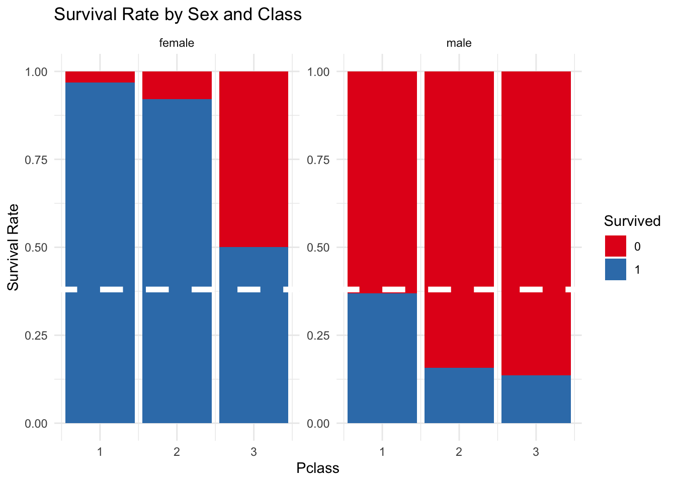
5.5.2) Cherborg, Sex and Class
The below graph splits the variables of port, sex and class to see how these variables impacted survival. Some interesting trends are identified.
Firstly, almost all the females from first and second class survived, regardless of the port where they started their journey. Females from third class did not have such luck with lower survival rates depending on which port they boarded the ship. Females from Southampton had a survival rate particularmente lower than the other females.
In relation to the male passengers there were higher survival rates for those who had boarded the boat in Southampton and Cherborg. Additionally, Cherborg had the highest male survival rate for each of the three classes. Finally, almost all of the males from Queenstown died, with third class males from this port having the highest survival rate from male Queenstown passengers.
ggplot(total %>% filter(group=="train"), aes(Embarked, fill = as.factor(Survived))) +

  facet_wrap(~Sex~Pclass, scale = "free") +

  geom_bar(position = "fill") +

  scale_fill_brewer(palette="Set1") +

  ylab("Survival Rate") +

  ggtitle("Survival Rate by Emarking Point") +

  labs(fill = "Survived") +

    geom_hline(yintercept=0.38, col="white", lty=2, size=2) +

  theme_minimal()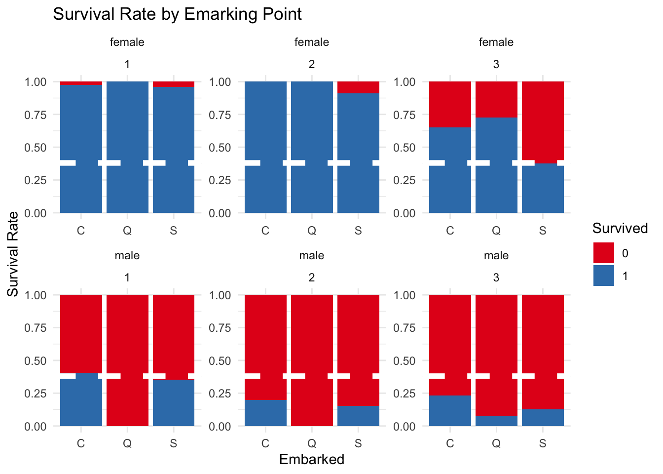
5.6) Family Size
In the below graph it is noted that families of two, three, or four people on the Titanic had a higher rate of survival.
ggplot(total %>% filter(group=="train"), aes(Family_size, fill=as.factor(Survived))) +

  geom_bar(position = "fill") +

  scale_fill_brewer(palette="Set1") +

  ylab("Survival Rate") +

  geom_hline(yintercept=0.38, col="white", lty=2, size=2) +

  ggtitle("Survival Rate by Family Size and Class") +

  labs(fill = "Survived") +

  theme_minimal()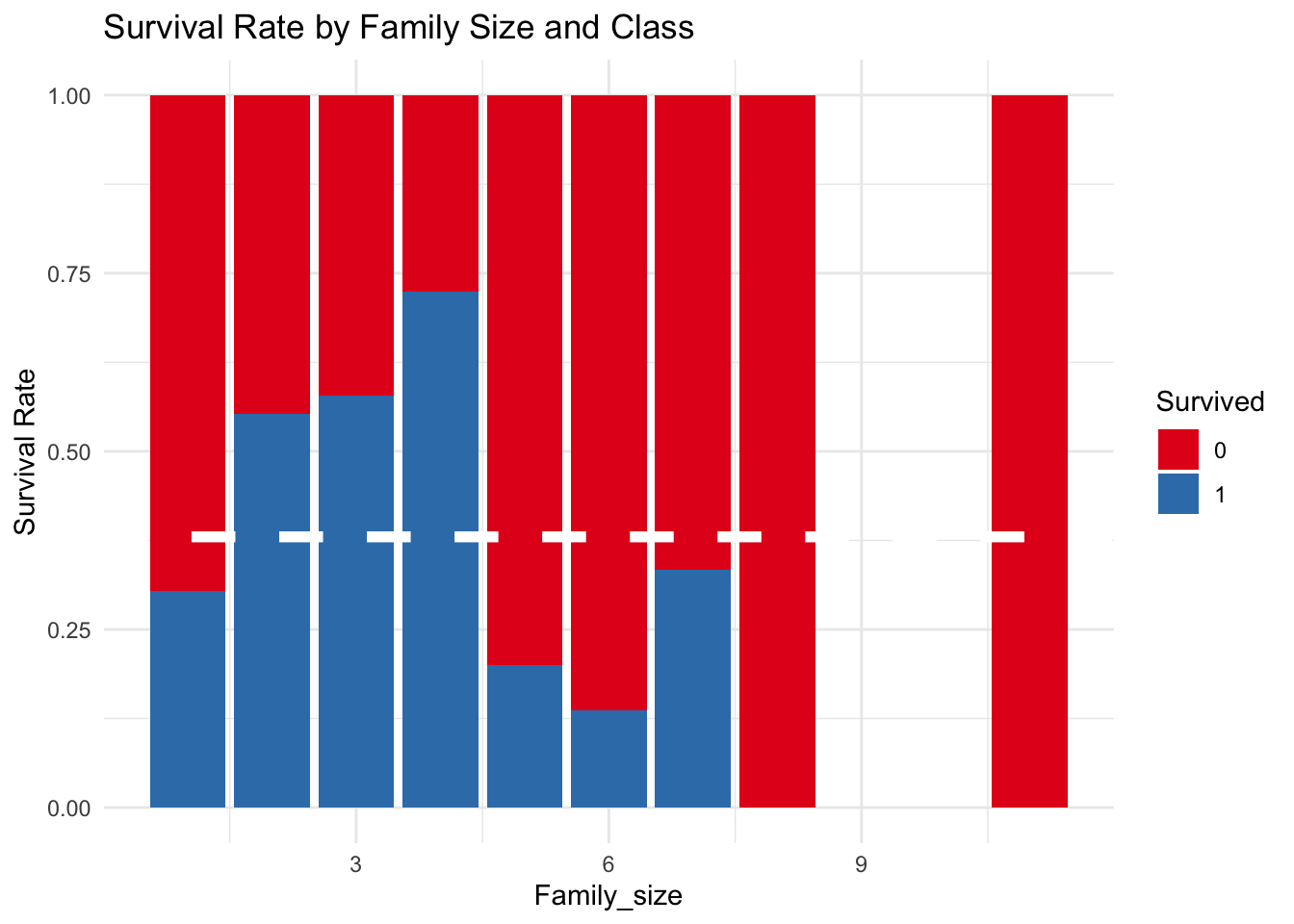
6) Creating the Model
6.1) Preparing the Data
Firstly, the variables used in the model need to be chosen. As previously explained, Fare and Cabin are not used. The train observations are put in a separate group and then divided into two separate groups:
train_val = 80% of the training observations
train_test_val = 20% of the training observations
The train_val is used to train the model. Then the model is tested firstly using the train_test_val. The results of this testing are used to adjust the model so that the best settings can be used when testing the model with the real test data.
Finally with the model adjusted the model is tested using the real test data with the dependent variable hidden.
feauter1 <-total[1:891, c("Pclass", "Title","Sex","Embarked","Family_size","Age Group", "Survived")]

feauter1$Survived <- as.factor(feauter1$Survived)

set.seed(500)

ind <- createDataPartition(feauter1$Survived,times=1,p=0.8,list=FALSE)

train_val <- feauter1[as.vector(ind),]

train_test_val <- feauter1[-ind,]
6.2) The Distribution of the Dependent Variable
The distribution of passengers that survived and died in the train_val and train_test_val groups will be analysed below to ensure that there is an equal distribution between the two groups. The distribution of survivors and fatalities across the groups is equal with a ratio of 6 deaths to 4 survivors.
round(prop.table(table(train$Survived)*100),digits = 1)##
## 0 1
## 0.6 0.4round(prop.table(table(train_val$Survived)*100),digits = 1)##
## 0 1
## 0.6 0.4round(prop.table(table(train_test_val$Survived)*100),digits = 1)##
## 0 1
## 0.6 0.46.3) Decision Tree Model
In this section a decision tree model is created using the train_val group which represents 54% of the total data. Then the train_test_val group is used to test and make adjustments to the model.
Having created the model the Confusion Matrix can be used to see its accuracy. The model has an accuracy of 0.8389 with a kappa of 0.642. Cross Validation is used to verify the model and to check that over fitting has not occurred.
set.seed(1234)

Model_DT <- rpart(Survived~.,data=train_val,method="class")

rpart.plot(Model_DT,extra =  3,fallen.leaves = T)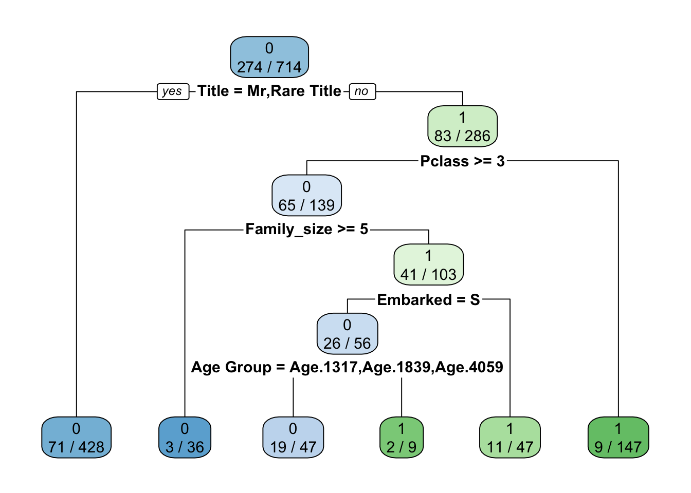
PRE_TDT=predict(Model_DT,data=train_val,type="class")

confusionMatrix(PRE_TDT,train_val$Survived)## Confusion Matrix and Statistics
##
## Reference
## Prediction 0 1
## 0 418 93
## 1 22 181
##
## Accuracy : 0.8389
## 95% CI : (0.8099, 0.8652)
## No Information Rate : 0.6162
## P-Value [Acc > NIR] : < 2.2e-16
##
## Kappa : 0.642
##
## Mcnemar's Test P-Value : 6.686e-11
##
## Sensitivity : 0.9500
## Specificity : 0.6606
## Pos Pred Value : 0.8180
## Neg Pred Value : 0.8916
## Prevalence : 0.6162
## Detection Rate : 0.5854
## Detection Prevalence : 0.7157
## Balanced Accuracy : 0.8053
##
## 'Positive' Class : 0
## 6.4) Cross Validation
Cross validation is used ten times to ensure that there is sufficient data being used to create the model and that it represents the full range of the complete data. With this method the train_val group is divided into ten parts. Each part is used as the test group once with the other nine parts being used as the training data. In this way it is less probable that over fitting occurs.
set.seed(1234)

cv.10 <- createMultiFolds(train_val$Survived, k = 10, times = 10)

# Control

ctrl <- trainControl(method = "repeatedcv", number = 10, repeats = 10,

                       index = cv.10)


train_val <- as.data.frame(train_val)

##Train the data

Model_CDT <- train(x = train_val[,-7], y = train_val[,7], method = "rpart", tuneLength = 30,

                   trControl = ctrl)


rpart.plot(Model_CDT$finalModel, type=4, clip.right.labs=FALSE, branch=.7)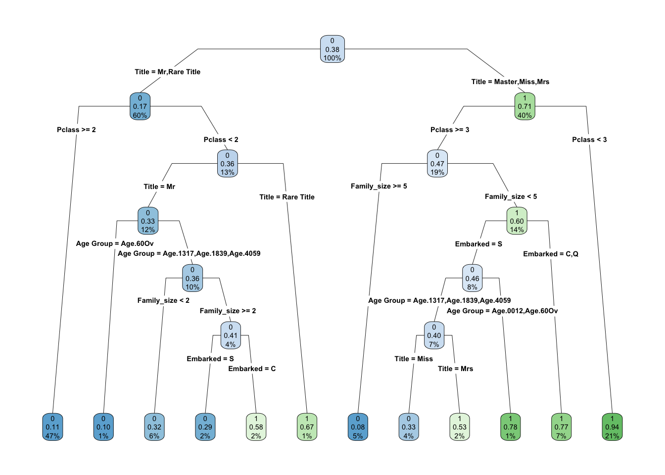
6.4.1) Cross Validation Predictions
The below confusion matrix shows how the cross validation model has a precision of 0.8079. This is less that the accuracy of the first model created which did not use cross validation (accuracy of 0.8389). This suggests that over fitting did occur in the first model.
set.seed(1234)
PRE_VDTS=predict(Model_CDT$finalModel,newdata=train_test_val,type="class")

confusionMatrix(PRE_VDTS,train_test_val$Survived)## Confusion Matrix and Statistics
##
## Reference
## Prediction 0 1
## 0 94 19
## 1 15 49
##
## Accuracy : 0.8079
## 95% CI : (0.7421, 0.8632)
## No Information Rate : 0.6158
## P-Value [Acc > NIR] : 2.854e-08
##
## Kappa : 0.5895
##
## Mcnemar's Test P-Value : 0.6069
##
## Sensitivity : 0.8624
## Specificity : 0.7206
## Pos Pred Value : 0.8319
## Neg Pred Value : 0.7656
## Prevalence : 0.6158
## Detection Rate : 0.5311
## Detection Prevalence : 0.6384
## Balanced Accuracy : 0.7915
##
## 'Positive' Class : 0
## rpart.rules(Model_CDT$finalModel)## .outcome
## 0.08 when Title is Master or Miss or Mrs & Pclass >= 3 & Family_size >= 5
## 0.10 when Title is Mr & Pclass < 2 & Age Group is Age.60Ov
## 0.11 when Title is Mr or Rare Title & Pclass >= 2
## 0.29 when Title is Mr & Pclass < 2 & Family_size >= 2 & Age Group is Age.1317 or Age.1839 or Age.4059 & Embarked is S
## 0.32 when Title is Mr & Pclass < 2 & Family_size < 2 & Age Group is Age.1317 or Age.1839 or Age.4059
## 0.33 when Title is Miss & Pclass >= 3 & Family_size < 5 & Age Group is Age.1317 or Age.1839 or Age.4059 & Embarked is S
## 0.53 when Title is Mrs & Pclass >= 3 & Family_size < 5 & Age Group is Age.1317 or Age.1839 or Age.4059 & Embarked is S
## 0.58 when Title is Mr & Pclass < 2 & Family_size >= 2 & Age Group is Age.1317 or Age.1839 or Age.4059 & Embarked is C
## 0.67 when Title is Rare Title & Pclass < 2
## 0.77 when Title is Master or Miss or Mrs & Pclass >= 3 & Family_size < 5 & Embarked is C or Q
## 0.78 when Title is Master or Miss or Mrs & Pclass >= 3 & Family_size < 5 & Age Group is Age.0012 or Age.60Ov & Embarked is S
## 0.94 when Title is Master or Miss or Mrs & Pclass < 36.5) Important Variables
The importance of the variables in both models is shown below. In both models, title and gender are the most important variables in determining whether someone survived or not.
This trend is reflected in the analysis carried out in Section 5 of this publication with males and passengers with the title of ‘Mr’ having a very low rate of survival.
# Get importance
Model_DT$variable.importance
## Title Sex Family_size Pclass Age Group Embarked
## 111.41503 96.41472 54.63255 31.71858 28.20113 11.29332Model_CDT$finalModel$variable.importance## Title Sex Family_size Pclass Age Group Embarked
## 114.23647 97.02466 55.44293 40.43166 29.94150 12.492176.6) Final Testing
In this section the model is tested using the original testing data with its hidden results for the dependent variable. The model with cross validation is used.
Running this model against the test data it is predicted that out of 418 passengers, 258 died, and 160 survived giving a survival rate of 38.28 percent, which is very close to the survival rate of 38.38% for the training data.
set.seed(1234)
PRE_TEST=predict(Model_CDT$finalModel,newdata=total[892:1309,],type="class")

PRE_TEST## 1 2 3 4 5 6 7 8 9 10 11 12 13 14 15 16 17 18 19 20
## 0 1 0 0 1 0 1 0 1 0 0 0 1 0 1 1 0 0 0 1
## 21 22 23 24 25 26 27 28 29 30 31 32 33 34 35 36 37 38 39 40
## 1 1 1 1 1 0 1 0 0 0 0 0 1 1 1 0 0 0 0 0
## 41 42 43 44 45 46 47 48 49 50 51 52 53 54 55 56 57 58 59 60
## 0 0 0 1 1 0 0 0 1 1 0 0 1 1 0 0 0 0 0 1
## 61 62 63 64 65 66 67 68 69 70 71 72 73 74 75 76 77 78 79 80
## 0 0 0 1 1 1 1 0 0 1 1 0 0 0 1 0 0 1 0 1
## 81 82 83 84 85 86 87 88 89 90 91 92 93 94 95 96 97 98 99 100
## 1 0 0 0 0 0 1 0 1 1 1 0 1 0 0 0 1 0 0 0
## 101 102 103 104 105 106 107 108 109 110 111 112 113 114 115 116 117 118 119 120
## 1 0 0 0 1 0 0 0 0 0 0 1 1 1 1 0 0 1 0 1
## 121 122 123 124 125 126 127 128 129 130 131 132 133 134 135 136 137 138 139 140
## 1 0 1 0 0 0 0 1 0 0 0 1 0 0 0 0 0 0 0 0
## 141 142 143 144 145 146 147 148 149 150 151 152 153 154 155 156 157 158 159 160
## 0 1 0 0 0 0 0 0 0 0 1 0 0 1 0 0 1 0 0 1
## 161 162 163 164 165 166 167 168 169 170 171 172 173 174 175 176 177 178 179 180
## 1 1 1 0 0 1 0 0 1 0 0 0 0 0 0 1 1 1 1 1
## 181 182 183 184 185 186 187 188 189 190 191 192 193 194 195 196 197 198 199 200
## 0 1 1 0 1 0 1 0 0 0 0 0 1 0 1 0 1 0 0 1
## 201 202 203 204 205 206 207 208 209 210 211 212 213 214 215 216 217 218 219 220
## 1 1 1 1 0 0 1 0 1 0 0 0 0 1 0 0 1 0 1 0
## 221 222 223 224 225 226 227 228 229 230 231 232 233 234 235 236 237 238 239 240
## 1 0 1 0 1 1 0 1 0 0 0 1 0 0 1 0 0 0 1 1
## 241 242 243 244 245 246 247 248 249 250 251 252 253 254 255 256 257 258 259 260
## 1 1 1 0 1 0 1 0 1 1 1 0 1 0 0 0 0 0 1 0
## 261 262 263 264 265 266 267 268 269 270 271 272 273 274 275 276 277 278 279 280
## 0 0 1 1 0 0 0 0 0 0 0 0 1 1 0 1 0 0 0 0
## 281 282 283 284 285 286 287 288 289 290 291 292 293 294 295 296 297 298 299 300
## 0 1 1 1 1 0 0 0 0 0 0 1 0 1 0 0 1 0 0 0
## 301 302 303 304 305 306 307 308 309 310 311 312 313 314 315 316 317 318 319 320
## 0 0 0 0 1 1 0 1 0 1 0 0 0 1 1 1 1 0 0 0
## 321 322 323 324 325 326 327 328 329 330 331 332 333 334 335 336 337 338 339 340
## 0 0 0 0 1 0 1 0 0 0 1 0 0 1 0 0 0 0 0 1
## 341 342 343 344 345 346 347 348 349 350 351 352 353 354 355 356 357 358 359 360
## 0 0 0 1 1 0 0 1 0 1 1 0 0 0 1 0 1 0 0 1
## 361 362 363 364 365 366 367 368 369 370 371 372 373 374 375 376 377 378 379 380
## 0 1 1 0 1 0 0 0 1 0 0 1 0 0 1 1 0 0 0 0
## 381 382 383 384 385 386 387 388 389 390 391 392 393 394 395 396 397 398 399 400
## 0 0 1 1 0 1 0 0 0 0 0 1 1 0 0 1 0 1 0 0
## 401 402 403 404 405 406 407 408 409 410 411 412 413 414 415 416 417 418
## 1 0 1 0 1 0 0 1 1 1 1 1 0 0 1 0 0 1
## Levels: 0 1TEST_Results <- cbind(test, PRE_TEST)
summary(PRE_TEST)## 0 1
## 258 1607) Conclusion
In conclusion in this publication a decision tree model has been created to classify if passengers survived or died on the Titanic. The final model used cross validation in order to avoid over fitting.
When the model was tested against the train_test_val an accuracy of 80.79% was achieved.
Finally, when the model was tested using the test data it was predicted that out of the 418 test group passengers 258 died and 160 survived with a survival rate of 38.28%.
It would be interesting to extend this analysis in the future using a random forest model to see if the model accuracy could be improved.
Thanks you for reading this two part publication. Hopefully it has been informative.