Immigration - Where do they live? - Santiago
A few months ago an investigation was carried out by the author of StatCityPro into where immigrants live in Santiago de Chile. Various points of interest were identified regarding the number of immigrants and also where they lived upon arrival to Chile.
This publication looks to build on this previous work by looking at more current data from 2019 and also by using machine learning methods of classification to build a model to predict if immigrants live in the Eastern Sector of Santiago. More information can be read about the Eastern Sector.
2) Packages
The following packages will be used in this publication.
library(dplyr)
library(lubridate)
library(chilemapas)
library(ggplot2)
library(sf)
library(ggspatial)
library(caret)
library(modelr)
library(forcats)
library(caTools)
3) Data
The data used in this publication can be downloaded from the following link.
setwd("~/Documents/Machine Learning/4. Proyectos/Migration/Data Sets")

visas2019 <- read.csv("visas_otorgadas_2019.csv")
The below syntax can be used to reveal the data’s variables. In total there are 14 variables with 328,118 observations.
str(visas2019)## 'data.frame': 328115 obs. of 14 variables:
## $ SEXO : Factor w/ 2 levels "Femenino","Masculino": 2 1 1 2 2 2 2 2 2 1 ...
## $ PAÍS : Factor w/ 77 levels "Alemania","Angola",..: 58 65 65 18 65 31 18 14 14 14 ...
## $ NACIMIENTO : Factor w/ 26521 levels "","1900-01-01",..: 15106 16136 16461 14048 2870 17043 21235 16788 14639 15764 ...
## $ ACTIVIDAD : Factor w/ 14 levels "Dueña De Casa",..: 8 7 7 8 7 9 7 2 13 9 ...
## $ PROFESIÓN : Factor w/ 606 levels "A Bodega","A Planificac",..: 351 426 426 432 158 423 399 245 569 84 ...
## $ ESTUDIOS : Factor w/ 7 levels "Básico","Medio",..: 4 1 7 2 4 2 4 2 4 2 ...
## $ COMUNA : Factor w/ 340 levels "Algarrobo","Alhué",..: 304 113 262 327 127 308 304 10 91 113 ...
## $ PROVINCIA : Factor w/ 56 levels "Antártica Chilena",..: 49 49 49 56 25 51 49 2 49 49 ...
## $ REGIÓN : Factor w/ 16 levels "Antofagasta",..: 13 13 13 16 6 12 13 1 13 13 ...
## $ TIT_DEP : Factor w/ 3 levels "","D","T": 1 1 1 1 1 1 1 1 1 1 ...
## $ AUTORIDAD : Factor w/ 55 levels "Dem","Gobernación Antártica Chilena",..: 1 1 1 1 1 1 1 1 1 1 ...
## $ BENEFICIO_AGRUPADO: Factor w/ 7 levels "Estudiante","Inversionista",..: 5 5 5 5 5 5 5 5 5 5 ...
## $ AÑO : int 2019 2019 2019 2019 2019 2019 2019 2019 2019 2019 ...
## $ MES : int 4 7 7 7 5 2 2 5 6 5 ...4) Feature Engineering
Feature Engineering will be conducted to preapre the date for further analysis.
4.1) Filter Data
Firstly the data is filtered to only have data for the province of Santiago. From now on this area will be referred to as Santiago. It is important to note that this area does not include the comunas of San Bernado or Puente Alto as they are part of different provinces.
visas2019STG <- visas2019 %>% filter(REGIÓN == "Metropolitana de Santiago")

visas2019STG <- visas2019STG %>% filter(PROVINCIA == 'Santiago')
4.2) Missing Values
Some variables have a class of ‘No Informa’. However, this is not the case for TIT-DEP which has 15,902 without a value. In accordance with the other variables, a class of ‘No Informa’ is added for these missing values. After this all of the observations that have a value of ‘No Informa’ for any of the variables are removed from the data frame as they can reduce the precision of the model.
table(visas2019STG$ACTIVIDAD)

table(visas2019STG$PROFESIÓN)

table(visas2019STG$ESTUDIOS)

table(visas2019STG$TIT_DEP)

levels(visas2019STG$TIT_DEP)

levels(visas2019STG$TIT_DEP)[1] <- "No Informa"

table(visas2019STG$TIT_DEP)
visas2019STG <- visas2019STG %>% filter(!ACTIVIDAD == "No Informa" ) %>% filter(!PROFESIÓN == "No Informa") %>% filter(!ESTUDIOS == "No Informa") %>% filter(!TIT_DEP == "No Informa")4.3) Immigrante Age
The date of birth is converted to age.
visas2019STG$NACIMIENTO <- as.Date(visas2019STG$NACIMIENTO)

year <- 2020

Birth_year <- year(visas2019STG$NACIMIENTO)

visas2019STG <- visas2019STG %>% mutate(Age = year - Birth_year)
4.4) Geographic Coordinates
The package chilemapas is used to create a base map for the Province of Santiago.
Chile <- chilemapas::codigos_territoriales
STG <- Chile %>% filter(nombre_provincia == 'Santiago')
Comunas <- chilemapas::mapa_comunas
STGgeo <- left_join(STG, Comunas)
Additionally, accents are added to the names of each of the comunas, so that they can be combined with other data bases that use accents in their spelling of the comunas.
STGgeo[4, 2] = "Conchalí"
STGgeo[6, 2] = "Estación Central"
STGgeo[19, 2] = "Maipú"
STGgeo[20, 2] = "Ñuñoa"
STGgeo[22, 2] = "Peñalolén"
STGgeo[29, 2] = "San Joaquín"
STGgeo[31, 2] = "San Ramón"
The two data bases are combined.
visas2019STG <- visas2019STG %>% rename(nombre_comuna = COMUNA)

visas2019STG$nombre_comuna <- as.factor(visas2019STG$nombre_comuna)

visas2019STG <- left_join(visas2019STG, STGgeo)
5) Initial Analysis
In this section the data is explored.
5.1) Nationalities
In 2019 156,260 inmigrantes arrived to Santiago with a total of 76 nationalities. However, after following the feature engineering steps outline in Section 4 this number reduces to 98,655 with 76 nationalities. Of this amount Venezuelans are the most prominent representing 58.80% with 58,009 people. An additional point of interest is that of the ten most prominent nationalities eight are from South or Central America, with China and the United States the only exceptions. It is also observed that six of these ten nationalities speak Spanish as a first language.
visas2019STG %>% group_by(PAÍS) %>% count() %>% arrange(-n)## # A tibble: 75 x 2
## # Groups: PAÍS [75]
## PAÍS n
## <fct> <int>
## 1 Venezuela 58009
## 2 Perú 11474
## 3 Colombia 8465
## 4 Haití 7135
## 5 Bolivia 2424
## 6 Ecuador 2119
## 7 Argentina 1988
## 8 Brasil 1335
## 9 China 923
## 10 Estados Unidos 564
## # … with 65 more rows5.2) Where do they live?
The most popular comuna for immigrants in 2019 was Santiago Centro with 30,207 arrivals. This is not surprising as Santiago Centro is the center of the city where there is more access to services, employment opportunities and housing. However, it must be noted that the data used only refers to the comuna of residence when an immigrant applied for their visa. Therefore, it is possible that they have since moved to a different sector of the city as they have become used to the city and have developed a support network.
comuna_count <- visas2019STG %>% group_by(nombre_comuna) %>% count() %>% arrange(-n)

comuna_count
## # A tibble: 32 x 2
## # Groups: nombre_comuna [32]
## nombre_comuna n
## <chr> <int>
## 1 Santiago 30207
## 2 Estación Central 8080
## 3 Independencia 7291
## 4 Quinta Normal 4343
## 5 San Miguel 4124
## 6 Recoleta 3871
## 7 Ñuñoa 3736
## 8 Las Condes 3591
## 9 La Florida 3571
## 10 Maipú 2780
## # … with 22 more rowsThe total number of immigrants in each comuna is added to the STGgeo data frame so that it can be mapped below. Each comuna is labelled, with details of which comunas correspond to each number provided in the table below the map.
STGgeo <- left_join(STGgeo, comuna_count, by = "nombre_comuna")

STGgeo <- STGgeo %>% rename(number_inmigrantes = n)

STGgeo <- cbind(STGgeo, st_coordinates(st_centroid(STGgeo$geometry)))

labels <- seq(1,32)
ggplot() + geom_sf(data = STGgeo$geometry, aes(fill = STGgeo$number_inmigrantes)) +
scale_fill_viridis_c(option = "inferno",trans = 'sqrt') +
geom_text(data = STGgeo, aes(X, Y, label = labels), size = 3, color = "white") +
geom_text(data = STGgeo %>% filter(nombre_comuna == "Santiago"), aes(X, Y, label = "1"), size = 3, color = "black") +
annotation_north_arrow(aes(which_north = "true", location = "br"), pad_y = unit(0.8, "cm")) +
annotation_scale(aes(location = "br", style = "bar")) +
theme(panel.grid.major = element_line(color = gray(0.5), linetype = "dashed")) +
theme (panel.background = element_rect(fill = "light grey")) +
ggtitle("5.1) Location of immigrants that arrived in 2019") + xlab("Longitude") + ylab("Latitude") +
labs(fill = "Number of Immigrants")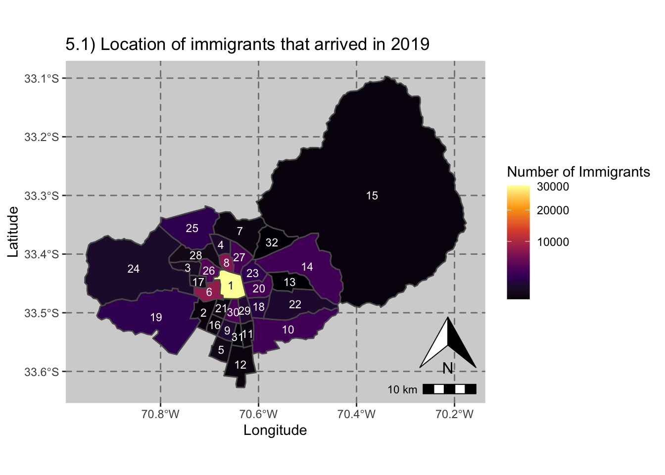
cbind(STGgeo, labels) %>% select(nombre_comuna, labels)## nombre_comuna labels
## 1 Santiago 1
## 2 Cerrillos 2
## 3 Cerro Navia 3
## 4 Conchalí 4
## 5 El Bosque 5
## 6 Estación Central 6
## 7 Huechuraba 7
## 8 Independencia 8
## 9 La Cisterna 9
## 10 La Florida 10
## 11 La Granja 11
## 12 La Pintana 12
## 13 La Reina 13
## 14 Las Condes 14
## 15 Lo Barnechea 15
## 16 Lo Espejo 16
## 17 Lo Prado 17
## 18 Macul 18
## 19 Maipú 19
## 20 Ñuñoa 20
## 21 Pedro Aguirre Cerda 21
## 22 Peñalolén 22
## 23 Providencia 23
## 24 Pudahuel 24
## 25 Quilicura 25
## 26 Quinta Normal 26
## 27 Recoleta 27
## 28 Renca 28
## 29 San Joaquín 29
## 30 San Miguel 30
## 31 San Ramón 31
## 32 Vitacura 325.4) The Eastern Sector
This publication and its part two counterpart aims to build a classification model to predict if an immigrant lives in the Eastern Sector. This sector contains the comunas of Providencia, Las Condes, Vitacura, and Lo Barnechea and is located to the north east of the city. These comunas are considered the most wealthy in the city and are identified in the below map.
SectorOriente <- STGgeo %>% filter(nombre_comuna == 'Providencia' | nombre_comuna == 'Las Condes' | nombre_comuna == 'Vitacura' | nombre_comuna == 'Lo Barnechea')

ggplot() + geom_sf(data = STGgeo$geometry, fill = "white") +
  geom_sf(data = SectorOriente$geometry, fill = "purple") +
geom_text(data = STGgeo, aes(X, Y, label = labels), size = 3, color = "white") +
annotation_north_arrow(aes(which_north = "true", location = "br"), pad_y = unit(0.8, "cm")) +
  annotation_scale(aes(location = "br", style = "bar")) +
  theme(panel.grid.major = element_line(color = gray(0.5), linetype = "dashed")) +
  theme (panel.background = element_rect(fill = "light grey")) +
  ggtitle("5.2 Eastern Sector of Santiago") + xlab("Longitude") + ylab("Latitude")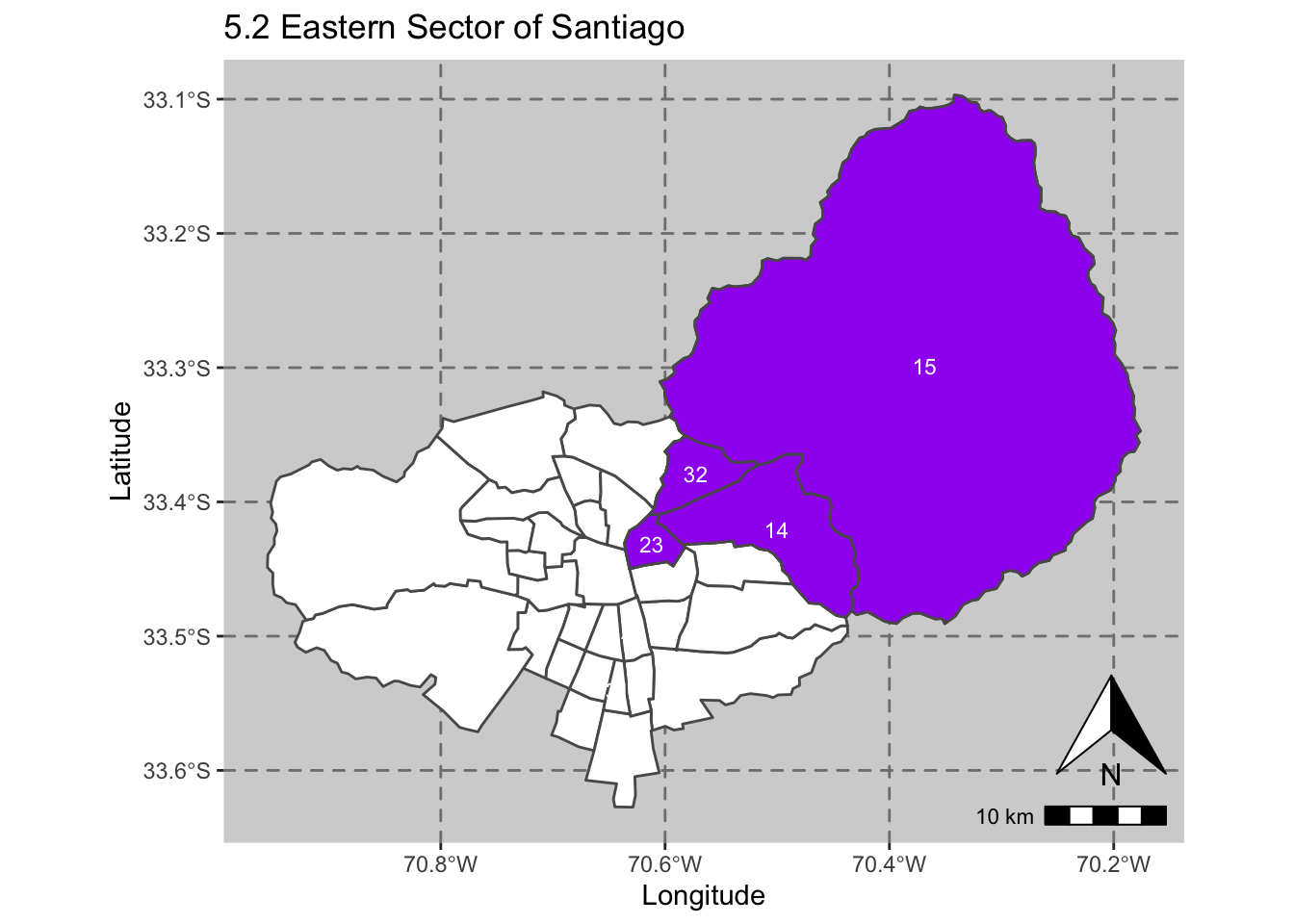
6) Further Mapping
In this section four maps are presented.
Map 6.1 shows the distribution of Venezuelan immigrants.
Map 6.2 shows the distribution of Haitian immigrants.
Map 6.3 shows the distribution of immigrants from the USA.
Map 6.4 shows the distribution of Peruvian immigrants.
These four nationalities were chosen as they play an important role in the immigration trends in Santiago. There has been a big increase in the number of Venezuelans in the last few years due to the political situation in their own country. The number of Haitians has also increased dramatically since 2015 due to the lower quality of life in their own country. The GDP per capita in Haiti is $868. This value is the lowest within the ten most prominent nationalities for immigrants that arrived to Santiago in 2019. Similarly it is interesting to explore the distribution of immigrants from the United States as it is the country with the highest GDP per capita. Finally, Peruvians are the nationality which historically has been the biggest contributor of immigrants to Chile. The GDP per capita (Banco Mundial, 2018) for each of the ten main nationalities are shown in US Dollars below.
USA = $62,887 Peru = $6,941 Colombia = $6,668 Haití = $868 Bolivia = $3,549 Ecuador = $6,345 Argentina = $11,684 Brasil = $9,001 China = $9,771
For comparison the GDP per capita of Chile is $15,923.
6.1) Venezuelans
This map shows that Venezuelans were concentrated in Santiago Centro with 21,387 people, corresponding to 36.88% of the Venezuelans that arrived in 2019. Estacion Central and Independencia were the second and third most populated comunas. In the eastern sector there were 1,998 Venezuelans.
venezuela_count <- visas2019STG %>% filter(PAÍS == 'Venezuela') %>% group_by(nombre_comuna) %>% count() %>% arrange(-n)

venezuela_count
## # A tibble: 32 x 2
## # Groups: nombre_comuna [32]
## nombre_comuna n
## <chr> <int>
## 1 Santiago 21387
## 2 Estación Central 5628
## 3 Independencia 4710
## 4 San Miguel 3318
## 5 Quinta Normal 2805
## 6 Ñuñoa 2622
## 7 La Florida 2339
## 8 Macul 1575
## 9 Maipú 1537
## 10 La Cisterna 1237
## # … with 22 more rowsvisas2019STG %>% filter(PAÍS == 'Venezuela' & nombre_comuna %in% c('Providencia', "Las Condes", 'Vitacura', 'Lo Barnechea')) %>% count()## n
## 1 1998STGgeo <- left_join(STGgeo, venezuela_count, by = "nombre_comuna")
STGgeo <- STGgeo %>% rename(numero_venezuelanos = n)ggplot() + geom_sf(data = STGgeo$geometry, aes(fill = STGgeo$numero_venezuelanos)) +
scale_fill_viridis_c(option = "inferno",trans = 'sqrt') +
geom_text(data = STGgeo, aes(X, Y, label = labels), size = 3, color = "white") +
annotation_north_arrow(aes(which_north = "true", location = "br"), pad_y = unit(0.8, "cm")) +
annotation_scale(aes(location = "br", style = "bar")) +
theme(panel.grid.major = element_line(color = gray(0.5), linetype = "dashed")) +
theme (panel.background = element_rect(fill = "light grey")) +
ggtitle("6.1 Location of Venezuelans that arrived in 2019") + xlab("Longitude") + ylab("Latitude") +
labs(fill = "Number of immigrants")
6.2) Haitians
The below map highlights that the most popular comuna for Haitians was Quilicura to the north of Santiago with 984 arrivals, accounting for 13.79% of the 7,135 Haitians that arrived in 2019. Estacion Central also had a high amount of Haitians with 758 arriving (10.62%). Likewise Santiago Centro had 523 (7.33%) arrivals. It is also interesting to note the lack of Haitians in the Eastern Sector of the city with only 25 Haitians arriving there in 2019.
haitiano_count <- visas2019STG %>% filter(PAÍS == 'Haití') %>% group_by(nombre_comuna) %>% count() %>% arrange(-n)

visas2019STG %>% filter(PAÍS == 'Haití') %>% count()
## n
## 1 7135haitiano_count## # A tibble: 32 x 2
## # Groups: nombre_comuna [32]
## nombre_comuna n
## <chr> <int>
## 1 Quilicura 984
## 2 Estación Central 758
## 3 Santiago 523
## 4 Lo Espejo 426
## 5 Recoleta 375
## 6 Pedro Aguirre Cerda 367
## 7 Cerro Navia 363
## 8 Conchalí 280
## 9 Quinta Normal 252
## 10 El Bosque 248
## # … with 22 more rowsvisas2019STG %>% filter(PAÍS == 'Haití' & nombre_comuna %in% c('Providencia', "Las Condes", 'Vitacura', 'Lo Barnechea')) %>% count()## n
## 1 25STGgeo <- left_join(STGgeo, haitiano_count, by = "nombre_comuna")
STGgeo <- STGgeo %>% rename(numero_haitianos = n)ggplot() + geom_sf(data = STGgeo$geometry, aes(fill = STGgeo$numero_haitianos)) +
scale_fill_viridis_c(option = "inferno",trans = 'sqrt') +
geom_text(data = STGgeo, aes(X, Y, label = labels), size = 3, color = "white") +
annotation_north_arrow(aes(which_north = "true", location = "br"), pad_y = unit(0.8, "cm")) +
annotation_scale(aes(location = "br", style = "bar")) +
theme(panel.grid.major = element_line(color = gray(0.5), linetype = "dashed")) +
theme (panel.background = element_rect(fill = "light grey")) +
ggtitle("6.2 Location of Haitians that arrived in 2019") + xlab("Longitude") + ylab("Latitude") +
labs(fill = "Number of immigrants")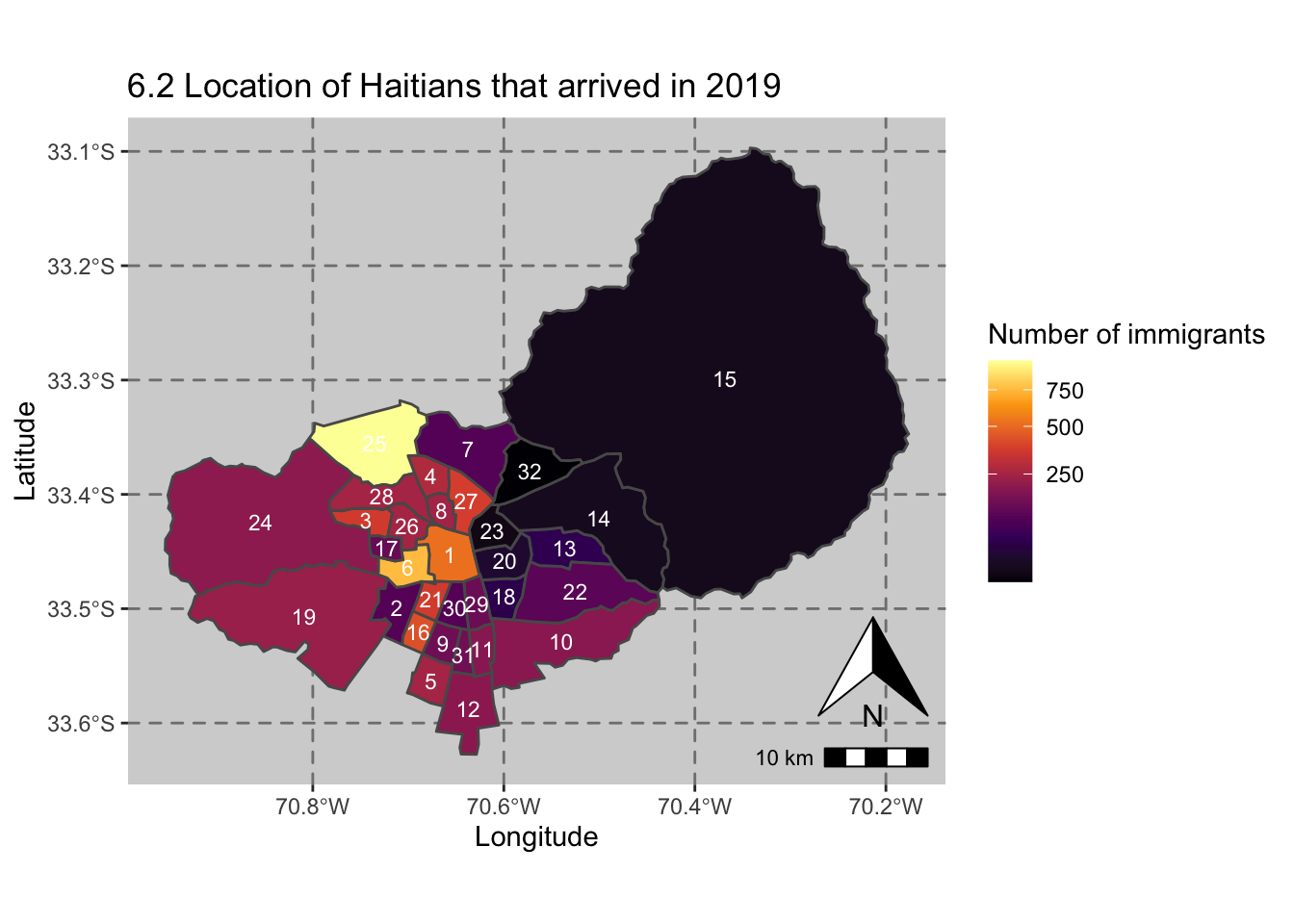
6.3) United States of America
Of the 564 US-Americans that arrived in 2019, 252 (62.41%) lived in the Eastern Sector. As was the case for Venezuelans and Haitians, Santiago Centro again received a high percentage of the arrivals with 80 people (14.18%). It is also interesting that there were various comunas without US-American arrivals in 2019, this was not the case for the other two nationalities analysed so far with Venezuelans and Haitians present in each of Santiago’s comunas.
eeuu_count <- visas2019STG %>% filter(PAÍS == 'Estados Unidos') %>% group_by(nombre_comuna) %>% count() %>% arrange(-n)

eeuu_count
## # A tibble: 23 x 2
## # Groups: nombre_comuna [23]
## nombre_comuna n
## <chr> <int>
## 1 Providencia 208
## 2 Las Condes 110
## 3 Santiago 80
## 4 Maipú 57
## 5 Ñuñoa 30
## 6 Vitacura 21
## 7 Lo Barnechea 13
## 8 Estación Central 11
## 9 Macul 5
## 10 Independencia 4
## # … with 13 more rowsvisas2019STG %>% filter(PAÍS == 'Estados Unidos') %>% count() ## n
## 1 564visas2019STG %>% filter(PAÍS == 'Estados Unidos' & nombre_comuna %in% c('Providencia', "Las Condes", 'Vitacura', 'Lo Barnechea')) %>% count()## n
## 1 352STGgeo <- left_join(STGgeo, eeuu_count, by = "nombre_comuna")
STGgeo <- STGgeo %>% rename(numero_eeuu = n)ggplot() + geom_sf(data = STGgeo$geometry, aes(fill = STGgeo$numero_eeuu)) +
scale_fill_viridis_c(option = "inferno",trans = 'sqrt') +
geom_text(data = STGgeo, aes(X, Y, label = labels), size = 3, color = "white") +
annotation_north_arrow(aes(which_north = "true", location = "br"), pad_y = unit(0.8, "cm")) +
annotation_scale(aes(location = "br", style = "bar")) +
theme(panel.grid.major = element_line(color = gray(0.5), linetype = "dashed")) +
theme (panel.background = element_rect(fill = "light grey")) +
ggtitle("6.3 Location of US-Americans that arrived in 2019") + xlab("Longitude") + ylab("Latitude") +
labs(fill = "Number of Immigrants")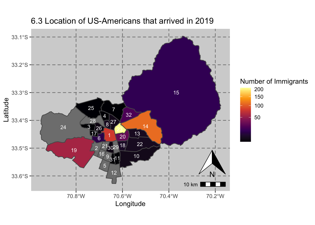
6.4) Peruvians
Santiago Centro, Recoleta, and Independencia were the three comunas with the most Peruvian arrivals in 2019 with 2,785 (24.27%), 1,272 (11.09%), and 1,092 (9.51%) respectively. In the Eastern Sector there were 855 (7.45%) Peruvians.
peruano_count <- visas2019STG %>% filter(PAÍS == 'Perú') %>% group_by(nombre_comuna) %>% count() %>% arrange(-n)

visas2019STG %>% filter(PAÍS == 'Perú') %>% count()
## n
## 1 11474visas2019STG %>% filter(PAÍS == 'Perú' & nombre_comuna %in% c('Providencia', "Las Condes", 'Vitacura', 'Lo Barnechea')) %>% count()## n
## 1 855peruano_count## # A tibble: 32 x 2
## # Groups: nombre_comuna [32]
## nombre_comuna n
## <chr> <int>
## 1 Santiago 2785
## 2 Recoleta 1272
## 3 Independencia 1092
## 4 Estación Central 634
## 5 Quinta Normal 585
## 6 Conchalí 475
## 7 Peñalolén 415
## 8 Las Condes 373
## 9 La Florida 335
## 10 Lo Prado 320
## # … with 22 more rowsSTGgeo <- left_join(STGgeo, peruano_count, by = "nombre_comuna")
STGgeo <- STGgeo %>% rename(numero_peruanos = n)ggplot() + geom_sf(data = STGgeo$geometry, aes(fill = STGgeo$numero_peruanos)) +
scale_fill_viridis_c(option = "inferno",trans = 'sqrt') +
geom_text(data = STGgeo, aes(X, Y, label = labels), size = 3, color = "white") +
annotation_north_arrow(aes(which_north = "true", location = "br"), pad_y = unit(0.8, "cm")) +
annotation_scale(aes(location = "br", style = "bar")) +
theme(panel.grid.major = element_line(color = gray(0.5), linetype = "dashed")) +
theme (panel.background = element_rect(fill = "light grey")) +
ggtitle("6.4 Location of Peruvians tha arrived in 2019") + xlab("Longitude") + ylab("Latitude") +
labs(fill = "Number of immigrants")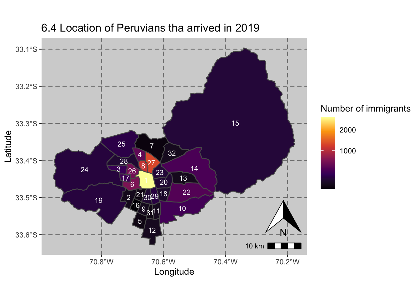
6.5) Analysis Summary
The following conclusions can be taken from the above analysis:
- There were more immigrants from Central America and South America.
- Speaking Spanish is an important factor for determining if there are many immigrants from a certain nationality.
- US-Americans have the highest GDP per capita and were the only analysed nationality with the majority of their population living in the Eastern Sector.
- Haitians have the lowest GDP per capita and also had the lowest percentage of people living in the Eastern Sector.
- Haitians were more widely dispersed with Quilicura, to the north of Santiago having the most Haitians. In comparison Venezuelans, US-Americans, and Peruvians were more concentrated around the center of the city.
7) Conclusion
In this part 1 publication immigration data from 2019 for Santiago has been explored with maps created for the distribution of Venezuelan, Haitian, US-American, and Peruvian immigrants, with some conclusions drawn. A part 2 publication will follow where a classification model will be created to try and classify if an immigrant lives in the Eastern Sector of the city. Thank you for reading this publication.