Immigration - Where do they live? - Part 2
This publication follows on from a previous post and looks to build a machine learning classification model to predict if an immigrant that arrived to Santiago de Chile in 2019 lived in the Eastern Sector of the city upon arrival.
Packages
The following packages are used in this publication.
library(dplyr)
library(caret)
library(modelr)
library(forcats)
library(caTools)
library(readr)
2) The Eastern Sector
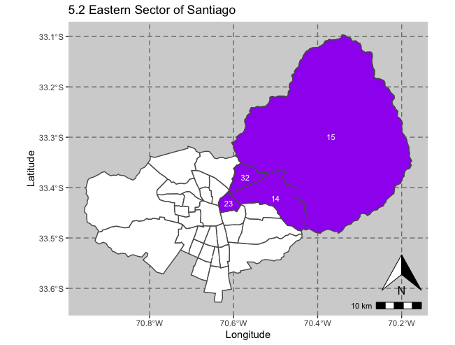
As previously explained the Eastern Sector contains the comunas of Providencia, Las Condes, Vitacura, y Lo Barnechea and is located to the north east of the city. These comunas are considered the most wealthy in the city and are identified in the below map.
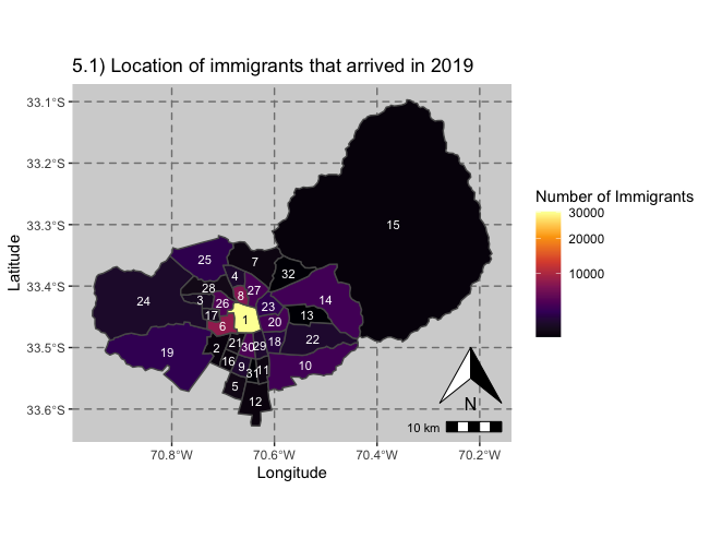
3) Distribution of Immigrants
The below map shows the distribution of all immigrants who arrived to Santiago in 2019. Tt must be noted that the data used only refers to the comuna of residence when an immigrant applied for their visa. Therefore, it is possible that they have since moved to a different sector of the city.
maplabels <- read_csv("lables.csv")## Warning: Missing column names filled in: 'X1' [1]## Parsed with column specification:
## cols(
## X1 = col_double(),
## nombre_comuna = col_character(),
## labels = col_double()
## )maplabels## # A tibble: 32 x 3
## X1 nombre_comuna labels
## <dbl> <chr> <dbl>
## 1 1 Santiago 1
## 2 2 Cerrillos 2
## 3 3 Cerro Navia 3
## 4 4 Conchalí 4
## 5 5 El Bosque 5
## 6 6 Estación Central 6
## 7 7 Huechuraba 7
## 8 8 Independencia 8
## 9 9 La Cisterna 9
## 10 10 La Florida 10
## # … with 22 more rows4) Data
The idea of this section is to create a classification model to predict in which comuna immigrants lived when they arrived to Santiago. The data used is the visas2019STG data frame that was prepared in part 1.
visas2019STG <- read.csv("visas2019STG.csv")5) Model Preparation
The following processes are conducted to prepare the data for modeling.
5.1) Selecting Variables and Eastern Sector Variable
First the relevant variables are choosen.
visas2019STGfilter <- visas2019STG %>% select(SEXO, PAÍS, ACTIVIDAD, PROFESIÓN, ESTUDIOS, nombre_comuna, AÑO, MES, Age)Second a new binomial variable is created to determine if an immigrant lived in the Eastern Sector. Within this variable 1 represents an immigrant that lived in the Eastern Sector, and 0 represents an immigrant who lived in a different sector of the city.
visas2019STGfilter$SECTOR_ORRIENTE <- if_else(visas2019STGfilter$nombre_comuna == 'Providencia', 1,
                                 if_else(visas2019STGfilter$nombre_comuna == 'Las Condes', 1,
                                         if_else(visas2019STGfilter$nombre_comuna == 'Vitacura', 1,
                                                 if_else(visas2019STGfilter$nombre_comuna =='Lo Barnechea', 1, 0))))
5.2) One Hot Encoding
Thirdly One Hot Encoding is conducted. This is a process by which to convert categorical variables into a strucutre which is easier to compute. When One Hot Encoding is applied to a particular variable, new columns are created for each categorical class of the original variable. For each class column, a one is recorded for all the observations that have that class, with a zero recorded for all those that do not.
One Hot Encoding is carried out for the variables of Sex, Activity and Studies.
Sex
model_matrix(visas2019STGfilter, SECTOR_ORRIENTE~SEXO-1)

visas2019STGfilter <- cbind(visas2019STGfilter, model_matrix(visas2019STGfilter, SECTOR_ORRIENTE~SEXO-1))
Activity
model_matrix(visas2019STGfilter, SECTOR_ORRIENTE~ACTIVIDAD-1)

visas2019STGfilter <- cbind(visas2019STGfilter, model_matrix(visas2019STGfilter, SECTOR_ORRIENTE~ACTIVIDAD-1))
Studies
model_matrix(visas2019STGfilter, SECTOR_ORRIENTE~ESTUDIOS-1)

visas2019STGfilter <- cbind(visas2019STGfilter, model_matrix(visas2019STGfilter, SECTOR_ORRIENTE~ESTUDIOS-1))
5.3) Countries to Continents
In total there are 75 nationalities in the data. To make these easier to compute a new variable is created, grouping the nationalities into continents. One Hot Encoding is then carried out for this variable.
visas2019STGfilter$continente <- fct_collapse(visas2019STGfilter$PAÍS, Europe = c('Alemania', 'Austria', 'Bélgica', 'Bulgaria', 'Croacia', 'Dinamarca', 'Eslovaquia', 'España', 'Finlandia',
                                                 'Francia', 'Grecia', 'Holanda', 'Hungría', 'Inglaterra', 'Irlanda', 'Italia', 'Lituania', 'Noruega',
                                                 'Polonia', 'Portugal', 'República Checa', 'República De Bielorrusia', 'República De Serbia',
                                                 'Rumanía', 'Rusia', 'Suecia', 'Suiza', 'Ucrania'), Africa = c('Angola', 'Camerún', 'Egipto', 'Marruecos', 'República de Congo', 'Sudráfica'),
             Asia = c('Bangladesh', 'Corea del Sur', 'China', 'Filipinas', 'India', 'Indonesia', 'Irán', 'Israel', 'Japón',
                      'Jordania', 'Líbano', 'Malasia', 'Nepal', 'Pakistán', 'Palestina', 'Siria', 'Tailandia', 'Taiwan', 'Turquía'),
             SouthAmerica = c('Argentina', 'Bolivia', 'Brasil', 'Colombia', 'Ecuador', 'Paraguay', 'Perú', 'Uruguay', 'Venezuela'),
             CentralAmerica = c('Costa Rica', 'Cuba', 'El Salvador', 'Guatemala', 'Haití', 'Honduras', 'México', 'Nicaragua', 'Panamá','República Dominicana'),
             NorthAmerica = c('Canadá', 'Estados Unidos'), Other = c('Otro país'),
             Oceania = c('Australia', 'Nueva Zelanda'))
visas2019STGfilter <- cbind(visas2019STGfilter, model_matrix(visas2019STGfilter, SECTOR_ORRIENTE~continente-1))6) Creating the Model
The data is divided into two groups. One is the training group with 75% of the observations. The second is the test group with 25% of the observations.
set.seed(1234)
split <- sample.split(visas2019STGfilter$SECTOR_ORRIENTE, SplitRatio = 0.75)
training_set <- subset(visas2019STGfilter, split == TRUE)
test_set <- subset(visas2019STGfilter, split == FALSE)
training_set_cut <- training_set[,c(-1, -2, -3, -4, -5, -6, -7, -8, -9, -34)]
test_set_cut <- test_set[,c(-1, -2, -3, -4, -5, -6, -7, -8, -9, -34)]6.2) Training the Model
A General Linear Model is used and trained with the below syntax.
set.seed(1234)
classifier = glm(formula = SECTOR_ORRIENTE ~.,
                  family = binomial,
                  data = training_set_cut)
The model is used to make predictions on the test data. A prediction of 1 represents an immigrant in the Eastern Sector and a prediction of 0 represents an immigrant in another area of the city. A Confusion Matrix is used to assess the accuracy of the model.
set.seed(1234)
prob_pred <- predict(classifier, type = 'response', newdata = test_set_cut[,c(-1)])
y_pred <- ifelse(prob_pred >= 0.5, 1, 0)cm <- confusionMatrix(factor(test_set_cut$SECTOR_ORRIENTE), factor(y_pred), positive = "1")
cm## Confusion Matrix and Statistics
##
## Reference
## Prediction 0 1
## 0 22616 169
## 1 1617 262
##
## Accuracy : 0.9276
## 95% CI : (0.9243, 0.9308)
## No Information Rate : 0.9825
## P-Value [Acc > NIR] : 1
##
## Kappa : 0.2042
##
## Mcnemar's Test P-Value : <2e-16
##
## Sensitivity : 0.60789
## Specificity : 0.93327
## Pos Pred Value : 0.13944
## Neg Pred Value : 0.99258
## Prevalence : 0.01747
## Detection Rate : 0.01062
## Detection Prevalence : 0.07618
## Balanced Accuracy : 0.77058
##
## 'Positive' Class : 1
## 7) Analysis
The confusion matrix compares the real data with the predicted data to show how accurate the model is. The matrix provides four values:
EasternSectorCorrect = 262
EasternSectorFalse = 1617
OtherSectorCorrect = 22616
OtherSectorIncorrect = 169

TotalObservations = EasternSectorCorrect + EasternSectorFalse + OtherSectorCorrect + OtherSectorIncorrect
The above values can be used to calculate the following four measures of model accuracy:
- Accuaracy
- Kappa
- Precision
- Recall
These values are discussed below.
7.1) Accuracy
The model had an accuracy of 92.76%. This means that the model classified 92.76% of the test data correctly.
Accuracy <- ((EasternSectorCorrect + OtherSectorCorrect)/TotalObservations)7.2) Precision
The model has a Precision of 13.94%. This means that of all the immigrants which the model predicted as living in the Easter Sector, 13.94% actually lived there.
Precision <- EasternSectorCorrect/(EasternSectorCorrect+EasternSectorFalse)7.3) Recall
The Recall value of 60.79% means that out of the 431 immigrants that actually lived in the Eastern Sector, the model correctly predicted that 60.79% of them lived there.
Recall <- EasternSectorCorrect / (EasternSectorCorrect + OtherSectorIncorrect)7.4) Kappa
One of the problems with the data is that it is not balanced. Only 431 immigrants from the test data live there accounting for 1.75%. Subsequently, the model can easily obtain a high accuracy as it could predict that all the observations do not live in the Eastern Sector, and it would still obtain an accuracy of 98.25%.
Therefore, the Kappa value can be used to measure how well the model performed. The models performance is compared with the results for if the model had been run at random on the data. The Kappa value is between 0 and 1, with the closer to 1 meaning the model is more accurate.
The model has a Kappa of 0.2042. This means that the model classifies the data with accuracy 20.42% better than that of random classification. A Kappa value of between 0.21 and 0.40 is considered reasonable. More can be read about how to calculate the Kappa value
6) Conclusion
In conclusion this publication has created a classification model to classifiy if an immigrant that arrived to Santiago in 2019 lived in the Eastern Sector. It has followed on from the part 1 publication which prepared the data and looked at the distribution of some nationalities throughout the city. When the model was used on the test data an accuracy of 92.76% was obtained with a Kappa value of 0.2042, suggesting that the model had some success. However, the Precision of 13.94% and the Recall value of 60.79% suggest that the model found it difficult to correctly classify immigrants from the Eastern Setor. The model could be improved with more equally spread data and different types of classification models. These options will be explored in future publications. Many thanks for reading this publication.