Covid 19 - Mapping Cases - Santiago

2) Packages

The following packages are used in this publication.

library(chilemapas)
library(ggplot2)
library(stringr)
library(tidyverse)
library(ggspatial)

3) Creating a Base Map

The package chilemapas is used to create a base map for the Metropolitan Region, in which Santiago resides. Additionally, accents are added to the names of each of the comunas, so that they can be combined with other data bases that use accents in their spelling of the comunas.

comunas <- chilemapas::mapa_comunas
codigos <- chilemapas::codigos_territoriales

comunas_info <- left_join(codigos, comunas)

comunas_info_RM <- comunas_info %>% filter(nombre_region == 'Metropolitana de Santiago')

comunas_info_RM[4, 2] = "Conchalí"
comunas_info_RM[6, 2] = "Estación Central"
comunas_info_RM[19, 2] = "Maipú"
comunas_info_RM[20, 2] = "Ñuñoa"
comunas_info_RM[22, 2] = "Peñalolén"
comunas_info_RM[29, 2] = "San Joaquín"
comunas_info_RM[31, 2] = "San Ramón"

ggplot() + geom_sf(data = comunas_info_RM$geometry) + ggtitle("Base Map of the Metropolitan Region") + ylab("Latitude") + xlab("Longitude")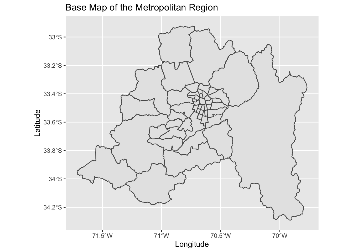

4) Data for Known Cases

The data for accumulated cases can be downloaded from the github of the Ministry of Health. With the data already downloaded it is loaded using the following syntax.

confirmedcases <- read_csv("~/Documents/Machine Learning/15. Hugo/academic-kickstart-master/content/en/post/MappingCovid/Covid-19_T.csv")

5) Feature Engineering

The objective of this section is to prepare the data so that it can be combined with the base map data in comunas_info_RM.

Firstly, the data is filtered so as to only include the comunas in the Metropolitan Region. Then the names in row two are made the variable names. Then rows one to four are removed.

The variables are converted to numerical variables.

RM %>% mutate_all(type.convert) %>%
    mutate_if(is.character, as.numeric) %>% 
  mutate_if(is.factor, as.Date)

## # A tibble: 37 x 54
##    Comuna     Alhue  Buin `Calera de Tang… Cerrillos `Cerro Navia` Colina
##    <date>     <dbl> <dbl>            <dbl>     <dbl>         <dbl>  <dbl>
##  1 2020-03-30     0     7                6         0            19     32
##  2 2020-04-01     0     8                7         4            21     39
##  3 2020-04-03     0    14                7         4            26     47
##  4 2020-04-06     0    20                7         5            31     50
##  5 2020-04-08     0    20                8        11            36     62
##  6 2020-04-10     0    29                8        21            42     66
##  7 2020-04-13     0    36               10        29            57     74
##  8 2020-04-15     0    40               10        39            65     77
##  9 2020-04-17     0    43               11        48            79     81
## 10 2020-04-20     0    47               14        53            99     90
## # … with 27 more rows, and 47 more variables: Conchali <dbl>, Curacavi <dbl>,
## #   `El Bosque` <dbl>, `El Monte` <dbl>, `Estacion Central` <dbl>,
## #   Huechuraba <dbl>, Independencia <dbl>, `Isla de Maipo` <dbl>, `La
## #   Cisterna` <dbl>, `La Florida` <dbl>, `La Granja` <dbl>, `La Pintana` <dbl>,
## #   `La Reina` <dbl>, Lampa <dbl>, `Las Condes` <dbl>, `Lo Barnechea` <dbl>,
## #   `Lo Espejo` <dbl>, `Lo Prado` <dbl>, Macul <dbl>, Maipu <dbl>, `Maria
## #   Pinto` <dbl>, Melipilla <dbl>, Nunoa <dbl>, `Padre Hurtado` <dbl>,
## #   Paine <dbl>, `Pedro Aguirre Cerda` <dbl>, Penaflor <dbl>, Penalolen <dbl>,
## #   Pirque <dbl>, Providencia <dbl>, Pudahuel <dbl>, `Puente Alto` <dbl>,
## #   Quilicura <dbl>, `Quinta Normal` <dbl>, Recoleta <dbl>, Renca <dbl>, `San
## #   Bernardo` <dbl>, `San Joaquin` <dbl>, `San Jose de Maipo` <dbl>, `San
## #   Miguel` <dbl>, `San Pedro` <dbl>, `San Ramon` <dbl>, Santiago <dbl>,
## #   Talagante <dbl>, Tiltil <dbl>, Vitacura <dbl>, `Desconocido
## #   Metropolitana` <dbl>

The data is filtered to only include two dates for each month, one on the 1st and one on the 15th. The data base is also converted from a wide format to a long format. Then the data base is divided by the date so as to have individual variables for each of the required dates. This process leaves the data in a matrix with a transformation to a data frame format being required. Additionally, here the excess date variables are deleted leaving only a variable for comuna and variables for the different dates. Then the variables are renamed and those which are numerical are converted to factors. Finally, row 9, which refers to cases with an unknown comuna, is removed.

RM_fechas <- RM %>% filter(Comuna %in% c('2020-03-30', '2020-04-15', '2020-05-01', '2020-05-15', '2020-06-01', '2020-06-15', '2020-07-01', 
                            '2020-07-13', '2020-07-24'))




RM_long <- RM_fechas %>%
  gather(key = "fecha",
         value = "Casos_Confirmados", 
         c(-Comuna))

RM_long %>% arrange(Comuna)

## # A tibble: 477 x 3
##    Comuna     fecha           Casos_Confirmados
##    <chr>      <chr>           <chr>            
##  1 2020-03-30 Alhue           0.0              
##  2 2020-03-30 Buin            7.0              
##  3 2020-03-30 Calera de Tango 6.0              
##  4 2020-03-30 Cerrillos       0.0              
##  5 2020-03-30 Cerro Navia     19.0             
##  6 2020-03-30 Colina          32.0             
##  7 2020-03-30 Conchali        14.0             
##  8 2020-03-30 Curacavi        5.0              
##  9 2020-03-30 El Bosque       18.0             
## 10 2020-03-30 El Monte        0.0              
## # … with 467 more rows

RM_long <- split(RM_long, RM_long$fecha)

class(RM_long)

## [1] "list"

RM_long <- data.frame(matrix(unlist(RM_long), nrow=length(RM_long), byrow=T))

RM_long <- RM_long[,18:27]


colnames(RM_long)[1:10] <- c("Comuna", '2020-03-30', '2020-04-15', '2020-05-01', '2020-05-15', '2020-06-01', '2020-06-15', '2020-07-01', '2020-07-13', '2020-07-24')

RM_long <- cbind(RM_long[,1], RM_long[,-1] %>% mutate_all(type.convert) %>%
    mutate_if(is.factor, as.numeric))

colnames(RM_long)[1] <- "Comuna"

RM_long <- RM_long[-9,]

Now the data for cases are combined with the base map data.

casos_en_comunas <- cbind(comunas_info_RM %>% arrange(nombre_comuna), RM_long)

6) Maps

Below there are varios maps showing how Covid 19 has spread in the Metropolitan Region. The data is for accumulated cases. Thank you for reading this publication and hopefully the maps are of interest and useful.

ggplot() + geom_sf(data = casos_en_comunas$geometry, aes(fill = casos_en_comunas$`2020-03-30`)) + 
  scale_fill_viridis_c(option = "inferno",trans = 'sqrt') +
  annotation_north_arrow(aes(which_north = "true", location = "br"), pad_y = unit(0.8, "cm")) +
  annotation_scale(aes(location = "br", style = "bar")) +
  theme(panel.grid.major = element_line(color = gray(0.5), linetype = "dashed")) +
  theme (panel.background = element_rect(fill = "light grey")) +
  ggtitle("Accumulated Confirmed Cases Covid 19 - 30 Marzo 2020 ") + xlab("Longitude") + ylab("Latitude") +
  labs(fill = "Number of Cases")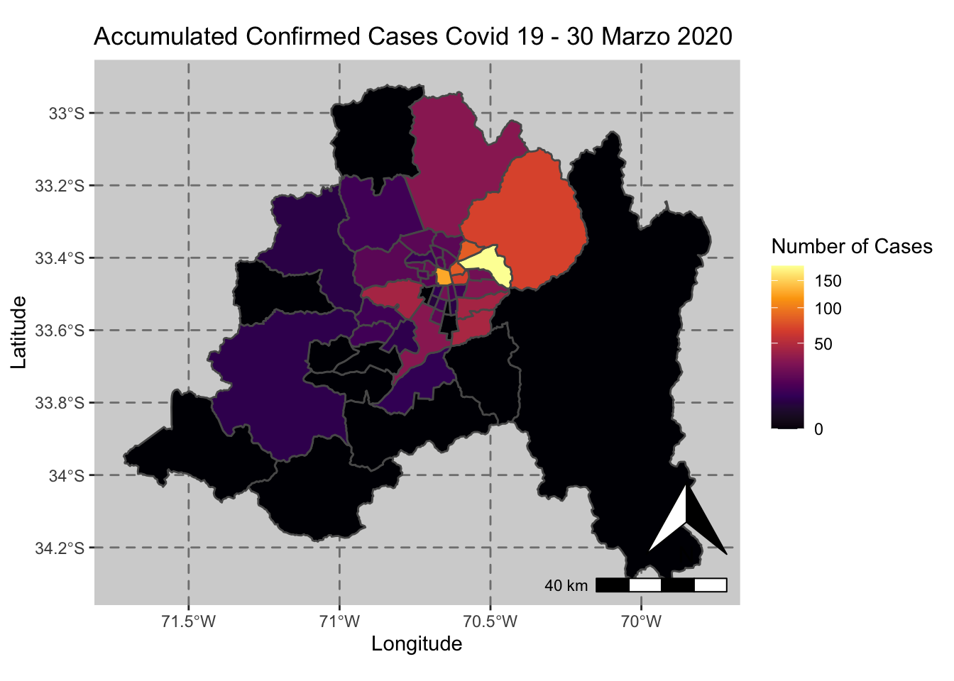

ggplot() + geom_sf(data = casos_en_comunas$geometry, aes(fill = casos_en_comunas$`2020-04-15`)) + 
  scale_fill_viridis_c(option = "inferno",trans = 'sqrt') +
  annotation_north_arrow(aes(which_north = "true", location = "br"), pad_y = unit(0.8, "cm")) +
  annotation_scale(aes(location = "br", style = "bar")) +
  theme(panel.grid.major = element_line(color = gray(0.5), linetype = "dashed")) +
  theme (panel.background = element_rect(fill = "light grey")) +
  ggtitle("Accumulated Confirmed Cases Covid 19 - 15 Abril 2020 ") + xlab("Longitude") + ylab("Latitude") +
  labs(fill = "Number of Cases")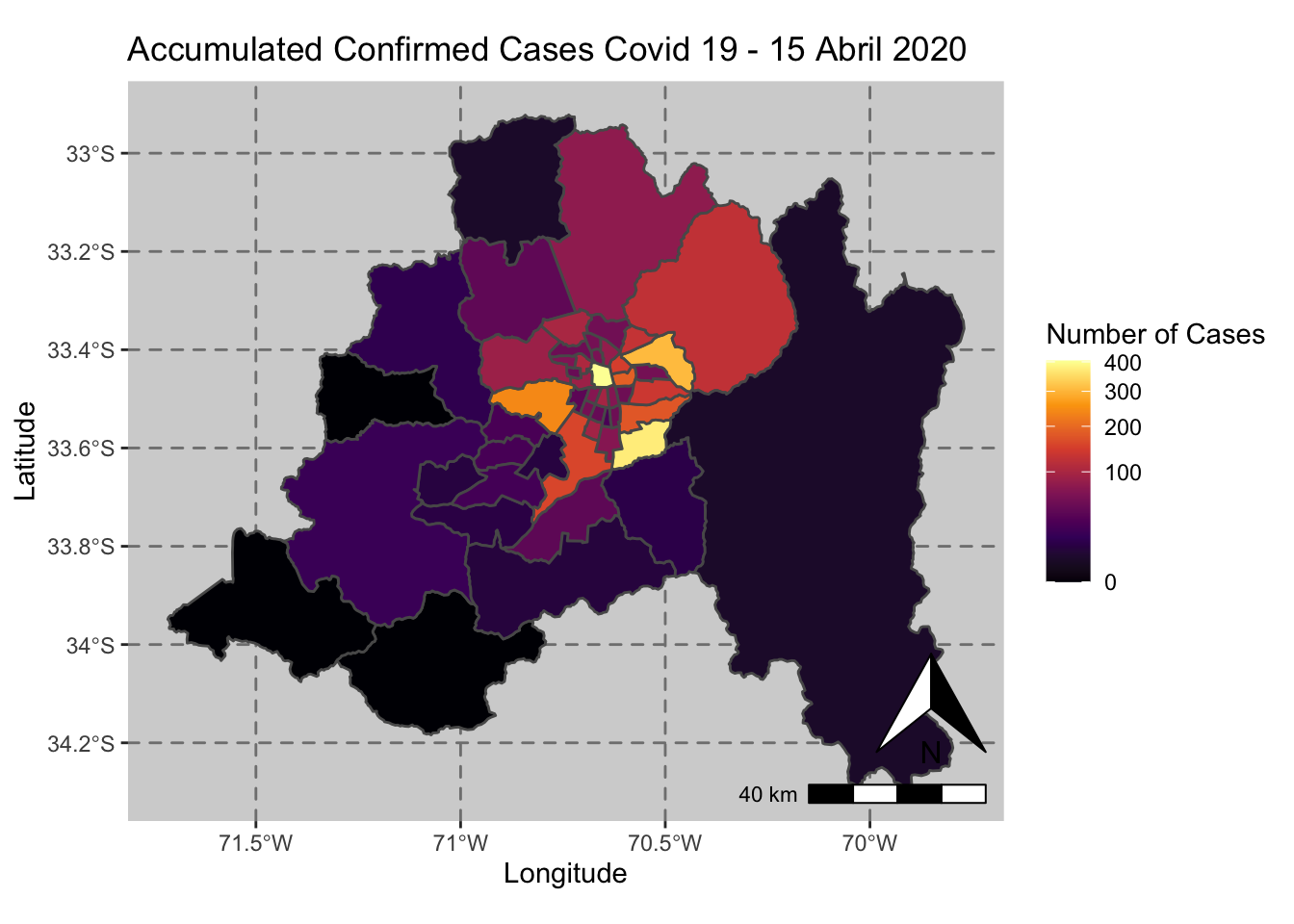

ggplot() + geom_sf(data = casos_en_comunas$geometry, aes(fill = casos_en_comunas$`2020-05-01`)) + 
  scale_fill_viridis_c(option = "inferno",trans = 'sqrt') +
  annotation_north_arrow(aes(which_north = "true", location = "br"), pad_y = unit(0.8, "cm")) +
  annotation_scale(aes(location = "br", style = "bar")) +
  theme(panel.grid.major = element_line(color = gray(0.5), linetype = "dashed")) +
  theme (panel.background = element_rect(fill = "light grey")) +
  ggtitle("Accumulated Confirmed Cases Covid 19 - 01 Mayo 2020 ") + xlab("Longitude") + ylab("Latitude") +
  labs(fill = "Number of Cases")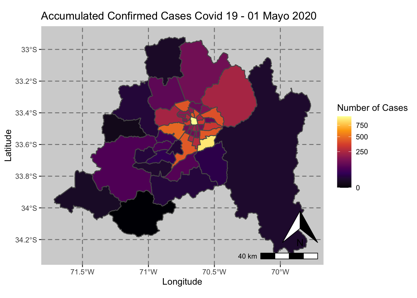

ggplot() + geom_sf(data = casos_en_comunas$geometry, aes(fill = casos_en_comunas$`2020-05-15`)) + 
  scale_fill_viridis_c(option = "inferno",trans = 'sqrt') +
  annotation_north_arrow(aes(which_north = "true", location = "br"), pad_y = unit(0.8, "cm")) +
  annotation_scale(aes(location = "br", style = "bar")) +
  theme(panel.grid.major = element_line(color = gray(0.5), linetype = "dashed")) +
  theme (panel.background = element_rect(fill = "light grey")) +
  ggtitle("Accumulated Confirmed Cases Covid 19 - 15 Mayo 2020 ") + xlab("Longitude") + ylab("Latitude") +
  labs(fill = "Number of Cases")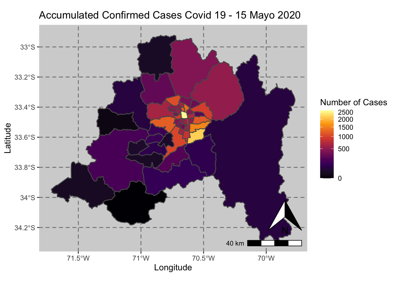

ggplot() + geom_sf(data = casos_en_comunas$geometry, aes(fill = casos_en_comunas$`2020-06-01`)) + 
  scale_fill_viridis_c(option = "inferno",trans = 'sqrt') +
  annotation_north_arrow(aes(which_north = "true", location = "br"), pad_y = unit(0.8, "cm")) +
  annotation_scale(aes(location = "br", style = "bar")) +
  theme(panel.grid.major = element_line(color = gray(0.5), linetype = "dashed")) +
  theme (panel.background = element_rect(fill = "light grey")) +
  ggtitle("Accumulated Confirmed Cases Covid 19 - 01 Junio 2020 ") + xlab("Longitude") + ylab("Latitude") +
  labs(fill = "Number of Cases")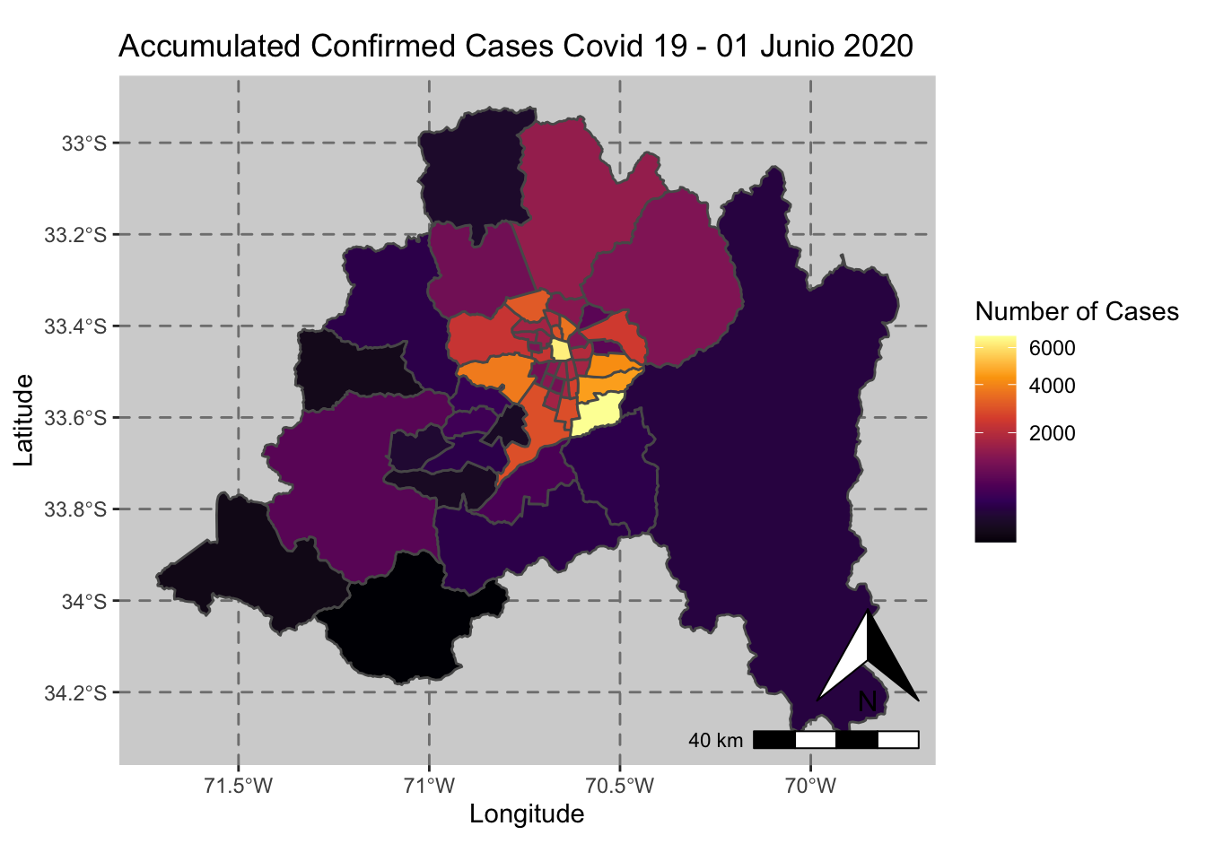

ggplot() + geom_sf(data = casos_en_comunas$geometry, aes(fill = casos_en_comunas$`2020-06-15`)) + 
  scale_fill_viridis_c(option = "inferno",trans = 'sqrt') +
  annotation_north_arrow(aes(which_north = "true", location = "br"), pad_y = unit(0.8, "cm")) +
  annotation_scale(aes(location = "br", style = "bar")) +
  theme(panel.grid.major = element_line(color = gray(0.5), linetype = "dashed")) +
  theme (panel.background = element_rect(fill = "light grey")) +
  ggtitle("Accumulated Confirmed Cases Covid 19 - 15 Junio 2020 ") + xlab("Longitude") + ylab("Latitude") +
  labs(fill = "Number of Cases")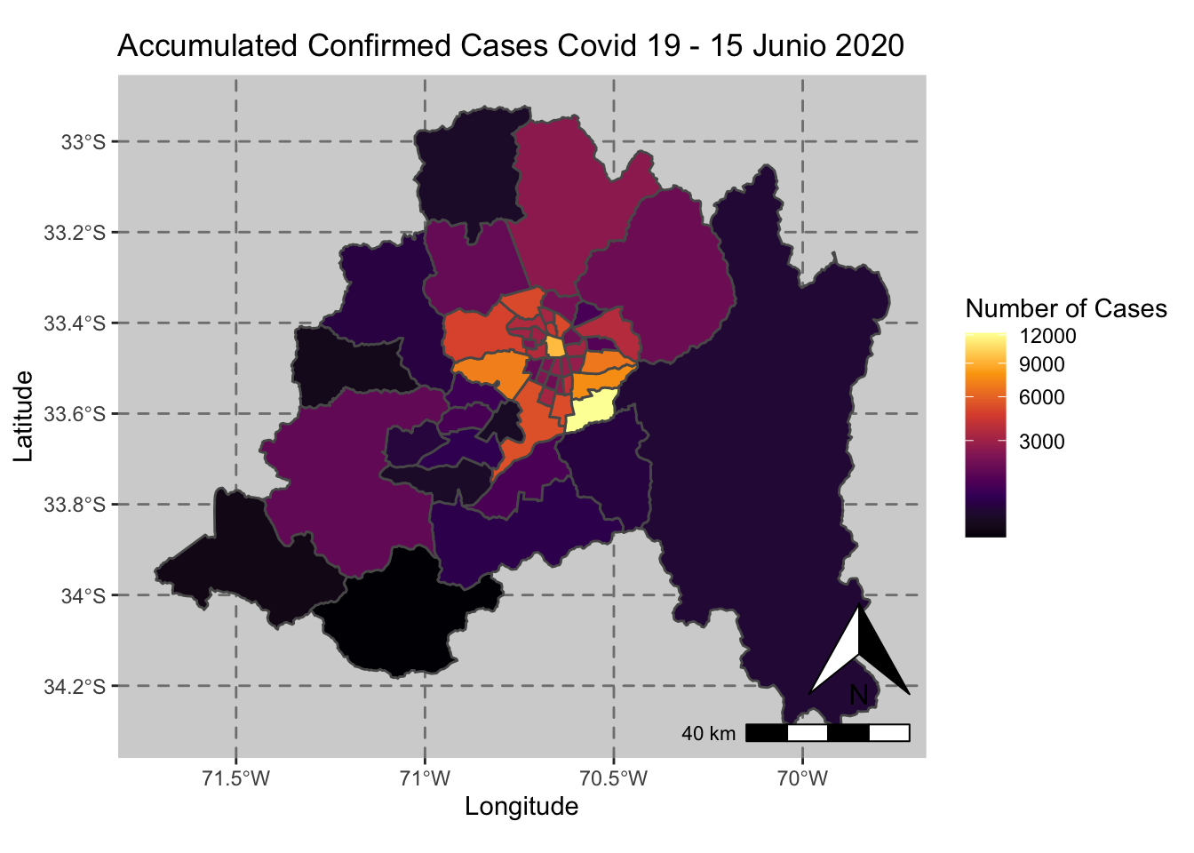

ggplot() + geom_sf(data = casos_en_comunas$geometry, aes(fill = casos_en_comunas$`2020-07-01`)) + 
  scale_fill_viridis_c(option = "inferno",trans = 'sqrt') +
  annotation_north_arrow(aes(which_north = "true", location = "br"), pad_y = unit(0.8, "cm")) +
  annotation_scale(aes(location = "br", style = "bar")) +
  theme(panel.grid.major = element_line(color = gray(0.5), linetype = "dashed")) +
  theme (panel.background = element_rect(fill = "light grey")) +
  ggtitle("Accumulated Confirmed Cases Covid 19 - 01 Julio 2020 ") + xlab("Longitude") + ylab("Latitude") +
  labs(fill = "Number of Cases")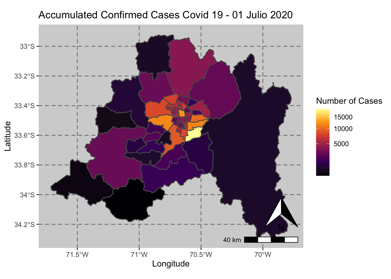

ggplot() + geom_sf(data = casos_en_comunas$geometry, aes(fill = casos_en_comunas$`2020-07-13`)) + 
  scale_fill_viridis_c(option = "inferno",trans = 'sqrt') +
  annotation_north_arrow(aes(which_north = "true", location = "br"), pad_y = unit(0.8, "cm")) +
  annotation_scale(aes(location = "br", style = "bar")) +
  theme(panel.grid.major = element_line(color = gray(0.5), linetype = "dashed")) +
  theme (panel.background = element_rect(fill = "light grey")) +
  ggtitle("Accumulated Confirmed Cases Covid 19 - 13 Julio 2020 ") + xlab("Longitude") + ylab("Latitude") +
  labs(fill = "Number of Cases")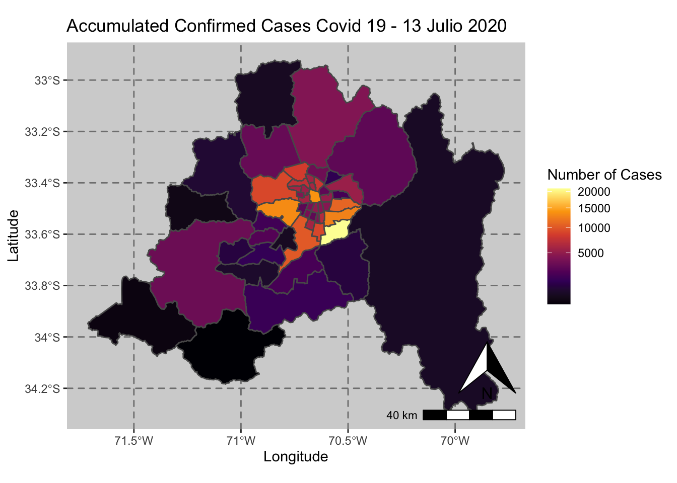

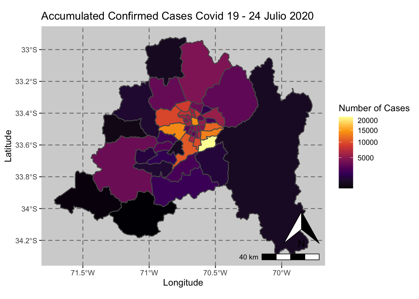
ggplot() + geom_sf(data = casos_en_comunas$geometry, aes(fill = casos_en_comunas$`2020-07-24`)) + 
  scale_fill_viridis_c(option = "inferno",trans = 'sqrt') +
  annotation_north_arrow(aes(which_north = "true", location = "br"), pad_y = unit(0.8, "cm")) +
  annotation_scale(aes(location = "br", style = "bar")) +
  theme(panel.grid.major = element_line(color = gray(0.5), linetype = "dashed")) +
  theme (panel.background = element_rect(fill = "light grey")) +
  ggtitle("Accumulated Confirmed Cases Covid 19 - 24 Julio 2020 ") + xlab("Longitude") + ylab("Latitude") +
  labs(fill = "Number of Cases")